Parallel Computing in R – Tips and tricks

Introduction

Traditionally, when we work with we use the sequential computing approach where instructions are processed one at a time, with each subsequent instruction waiting for the previous one to complete. It typically uses a single processor, which can result in lower performance and higher processor workload. The primary drawback of sequential computing is that it can be time-consuming, as only one instruction is executed at any given moment.

Parallel computing was introduced to overcome these limitations. In this approach, multiple instructions or processes are executed concurrently. By running tasks simultaneously, parallel computing saves time and is capable of solving larger problems. It uses multiple high-performance processors, which results in a lower workload for each processor.

What is a CPU?

The Central Processing Unit (CPU), also called processor, is a piece of computer hardware (electronic circuitry) that executes instructions, such as arithmetic, logic, controlling, and input/output (I/O) operations¹. In other words, it is the brain of the computer.

Modern CPUs consist of several units, named (physical) cores (multi-core processors). These cores can be multithreaded. This means that these cores can provide multiple threads of execution in parallel (usually up to 2). Threads are also known as logical cores.

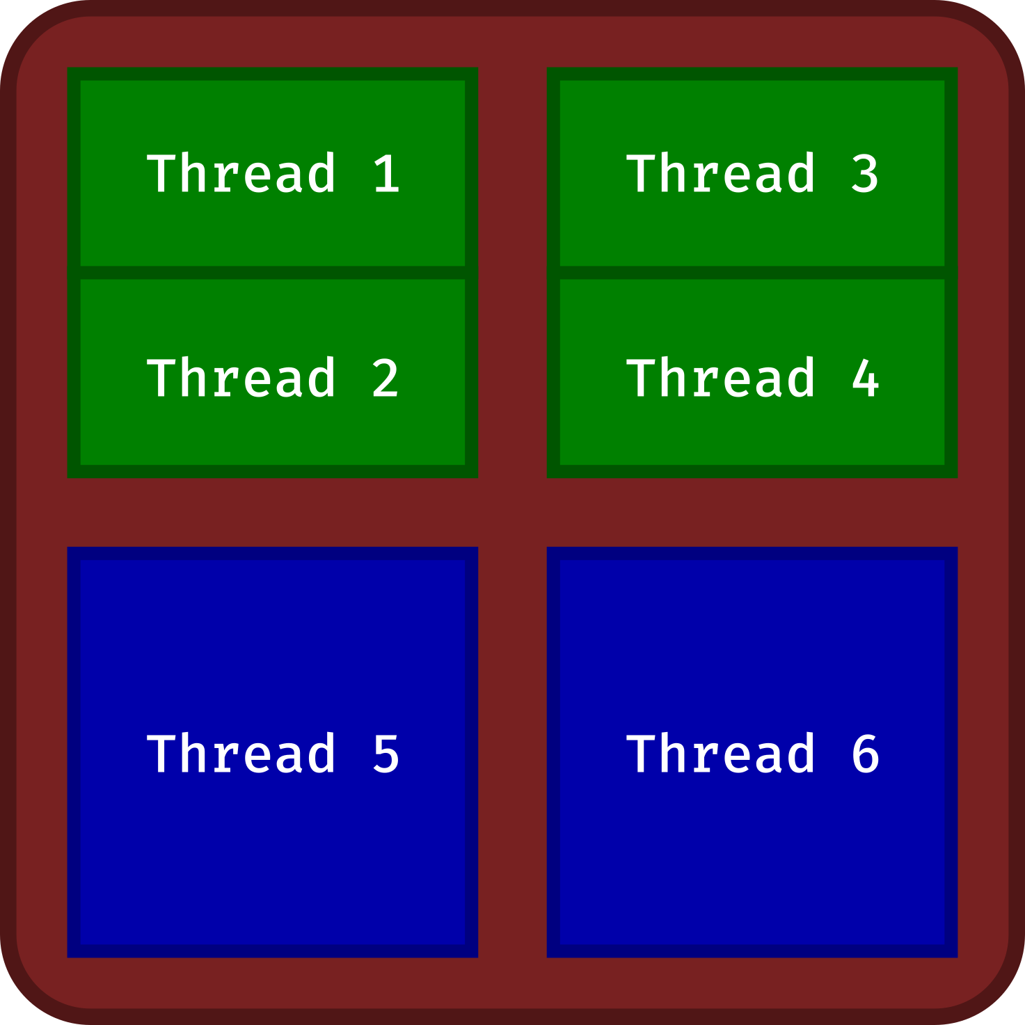
In this example, the CPU (in brown) contains 4 cores (in blue and green):

2 single-threading cores (in blue)
2 multi-threading cores (in green)

Six threads (logical cores) are available for parallel computing.

Note

For instance, my Lenovo P14s Gen 3 is shipped with the Intel® Core™ i7-1280P processor. It is made up of 6 multi-threading cores (2 threads per core) and 8 single-threading cores. Parallel computation can use 20 threads.

# How many logical cores are available on my computer?
parallel::detectCores(logical = TRUE)
## [1] 20

Parallel computing

Here we will focus on the Embarrassingly parallel computing paradigm. In this paradigm, a problem can be split into multiple independent pieces. The pieces of the problem are executed simultaneously as they don’t have to communicate with each other (except at the end when all outputs are assembled).

Hidden parallel tasks

Many packages (and system libraries) include built-in parallel computing that operates behind the scenes. This hidden parallel computing won’t interfere with your work and will actually enhance computational efficiency. However, it’s still a good idea to be aware of it, as it could impact other tasks (and users) using the same machine.

Data parallel computing involves splitting a large dataset into smaller segments and performing the same operation on each segment simultaneously. This approach is especially useful for tasks where the same computation must be applied to multiple data points (e.g. large data processing, simulations, machine learning, image and video processing).

Many packages implement high-performance and parallel computing (see this CRAN Task View).

The parallel package in implements two types of parallel computing:

Shared memory parallelization (or FORK): Each parallel thread is essentially a full copy of the master process, along with the shared environment, including objects and variables defined before the parallel threads are launched. This makes it run efficiently, especially when handling large datasets. However, a key limitation is that the approach does not work on Windows systems.
Distributed memory parallelization (or SOCKET): Each thread operates independently, without sharing objects or variables, which must be explicitly passed from the master process. As a result, it tends to run slower due to the overhead of communication. This approach is compatible with all operating systems.

Table: Comparison of two parallel computing approaches
	Forking	Socket
Operating system
Environment	Common to all sessions (time saving)	Unique to each session (transfer variables, functions & packages)
Usage	Very easy	More difficult (configure cluster & environment)

Source (in French): https://regnault.pages.math.cnrs.fr/meroo/src/quarto/calc_paral_R.html

Let’s explore these two approaches with a case study.

Case study

Objective: We want to intersect the spatial distribution of 40 species on a spatial grid (defining the Western Palearctic region) to create a matrix with grid cells in row and the presence/absence of each species in column.

The workflow is the following:

Import study area (grid)
Import species spatial distributions (polygons)
Subset polygons for species X
Intersect polygons X with the grid
Assemble occurrences of all species

Steps 3-4 must be repeated for each species and therefore can be parallelized.

Import data

Let’s import the study area, a regular spatial grid (sf POLYGONS) defined in the WGS84 system and delimiting the Western Palearctic region.

# Import study area ----
study_area  <- sf::st_read(file.path("data", "study_area.gpkg"))
study_area

Simple feature collection with 3254 features and 1 field
Geometry type: MULTIPOLYGON
Dimension:     XY
Bounding box:  xmin: -24.53429 ymin: 14.91196 xmax: 69.02288 ymax: 81.85871
Geodetic CRS:  WGS 84
First 10 features:
   id                           geom
1   1 MULTIPOLYGON (((11.46571 15...
2   2 MULTIPOLYGON (((11.46571 15...
3   3 MULTIPOLYGON (((12.46571 15...
4   4 MULTIPOLYGON (((13.46571 15...
5   5 MULTIPOLYGON (((14.46571 15...
6   6 MULTIPOLYGON (((15.46571 15...
7   7 MULTIPOLYGON (((16.46571 15...
8   8 MULTIPOLYGON (((17.46571 15...
9   9 MULTIPOLYGON (((26.46571 15...
10 10 MULTIPOLYGON (((26.46571 15...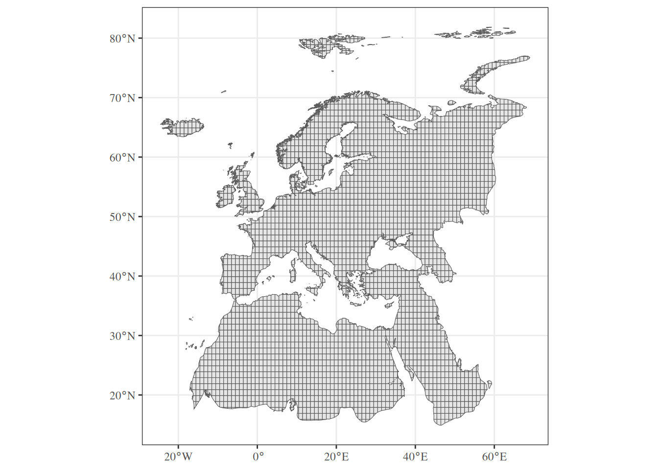

# Attach ggplot2 ----
library("ggplot2")

# Map study area ----
ggplot() +
  theme_bw() +
  theme(text = element_text(family = "serif")) +
  geom_sf(data = study_area)

Now let’s import the bird spatial distribution layer (sf POLYGONS) also defined in the WGS84 system.

# Import species distribution ----
sp_polygons <- sf::st_read(file.path("data", "species_polygons.gpkg"))
sp_polygons

Simple feature collection with 40 features and 1 field
Geometry type: MULTIPOLYGON
Dimension:     XY
Bounding box:  xmin: -30 ymin: 10 xmax: 75 ymax: 81.85748
Geodetic CRS:  WGS 84
First 10 features:
     binomial                           geom
1  species_01 MULTIPOLYGON (((6.04248 45....
2  species_02 MULTIPOLYGON (((-16.16014 2...
3  species_03 MULTIPOLYGON (((29.5531 40....
4  species_04 MULTIPOLYGON (((75 12.38982...
5  species_05 MULTIPOLYGON (((-7.675472 4...
6  species_06 MULTIPOLYGON (((-3.947759 4...
7  species_07 MULTIPOLYGON (((4.209473 36...
8  species_08 MULTIPOLYGON (((75 42.27599...
9  species_09 MULTIPOLYGON (((-4.051088 4...
10 species_10 MULTIPOLYGON (((5.534302 61...

Extract species names

Let’s extract the name of the 40 species (used later for parallel computing).

# Extract species names ----
sp_names <- unique(sp_polygons$"binomial")
sp_names <- sort(sp_names)
sp_names

 [1] "species_01" "species_02" "species_03" "species_04" "species_05"
 [6] "species_06" "species_07" "species_08" "species_09" "species_10"
[11] "species_11" "species_12" "species_13" "species_14" "species_15"
[16] "species_16" "species_17" "species_18" "species_19" "species_20"
[21] "species_21" "species_22" "species_23" "species_24" "species_25"
[26] "species_26" "species_27" "species_28" "species_29" "species_30"
[31] "species_31" "species_32" "species_33" "species_34" "species_35"
[36] "species_36" "species_37" "species_38" "species_39" "species_40"

Explore data

We will select polygons for species_22 and map layers.

# Subset one species ----
species      <- "species_22"
sub_polygons <- sp_polygons[sp_polygons$"binomial" == species, ]
sub_polygons

Simple feature collection with 1 feature and 1 field
Geometry type: MULTIPOLYGON
Dimension:     XY
Bounding box:  xmin: -6.235596 ymin: 52.44647 xmax: 34.74487 ymax: 71.18811
Geodetic CRS:  WGS 84
     binomial                           geom
22 species_22 MULTIPOLYGON (((5.123108 60...

# Map layers ----
ggplot() +
  theme_bw() +
  theme(text = element_text(family = "serif")) +
  geom_sf(data = study_area) +
  geom_sf(data = sub_polygons, 
          fill = "#4F000088", 
          col  = "#4F0000FF")

Define main function

Now let’s define a function that will report the occurrence of one species on the grid (step 4 of the workflow).

# Function to rasterize ----
polygon_to_grid <- function(grid, polygon) {

  ## Clean species name ----
  species <- unique(polygon$"binomial")
  species <- gsub(" ", "_", species) |> 
    tolower()
  
  ## Intersect layers ----
  cells <- sf::st_intersects(grid, polygon, sparse = FALSE)
  cells <- apply(cells, 1, any)
  cells <- which(cells)
  
  ## Create presence/absence column ----
  grid[     , species] <- 0
  grid[cells, species] <- 1
  
  ## Remove spatial information ----
  sf::st_drop_geometry(grid)
}

This function returns a data.frame with two columns: the identifier of the cell and the presence/absence of the species.

Test main function

Let’s try this function with the distribution of Curruca cantillans.

# Rasterize species polygons -----
sp_grid <- polygon_to_grid(study_area, sub_polygons)

although coordinates are longitude/latitude, st_intersects assumes that they
are planar

head(sp_grid)

  id species_22
1  1          0
2  2          0
3  3          0
4  4          0
5  5          0
6  6          0

# Add geometry ----
sf::st_geometry(sp_grid) <- sf::st_geometry(study_area)

# Convert occurrence to factor ----
sp_grid$"species_22" <- as.factor(sp_grid$"species_22")

# Map result ----
ggplot() +
  theme_bw() +
  theme(text = element_text(family = "serif"), legend.position = "none") +
  geom_sf(data    = sp_grid, 
          mapping = aes(fill = species_22)) +
  scale_fill_manual(values = c("0" = "#FFFFFFFF", 
                               "1" = "#9F0000FF"))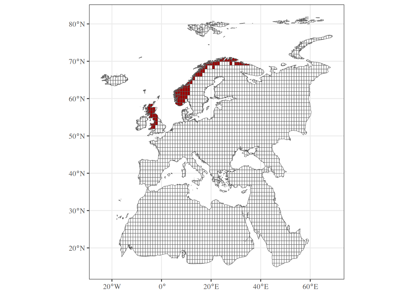

Our workflow is ready for one species. Now we have to apply this function on each species. Let’s have a look at different approaches.

Non-parallel: `for()` loop

One way of repeating a task is the iteration. Let’s walk over species with the for() loop.

# Create the output (list of 40 empty elements) ----
grids <- vector(mode = "list", length = length(sp_names))

# Define the sequence to loop on ----
for (i in 1:length(sp_names)) {
  
  # Instructions to repeat ----
  tmp <- sp_polygons[sp_polygons$"binomial" == sp_names[i], ]
  grd <- polygon_to_grid(study_area, tmp)
  
  # Store result in the output ----
  grids[[i]] <- grd

}

The output is a list of 40 data.frame.

Non-parallel: `lapply()`

Iterative computing is quite verbose and often time-consuming. Because is a functional programming language, we can wrap-up the body of the for() loop inside a function and apply this function over a vector (i.e. species names). Let’s illustrate this with the function lapply().

# lapply way ----
grids <- lapply(sp_names, function(sp) {
  
  tmp <- sp_polygons[sp_polygons$"binomial" == sp, ]
  grd <- polygon_to_grid(study_area, tmp)
  grd

})

The function lapply() also returns a list of 40 data.frame.

The purrr package

The purrr package provides an alternative to the apply() function family in base . For instance:

# purrr way ----
grids <- purrr::map(sp_names, function(sp) {
  
  tmp <- sp_polygons[sp_polygons$"binomial" == sp, ]
  grd <- polygon_to_grid(study_area, tmp)
  grd

})

The map() function of the purrr package returns the same output as lapply().

These three approaches work in a sequential way. It’s time to parallel our code to boost performance.

Forking: `mclapply()`

The parallel package provides the function mclapply(), a parallelized version of lapply(). Note that this function relies on the forking approach and doesn’t work on Windows.

# Required packages ----
library(parallel)

# Let's use 10 threads ----
n_cores <- 10

# mclapply way ----
grids <- mclapply(sp_names, function(sp) {
  
  tmp <- sp_polygons[sp_polygons$"binomial" == sp, ]
  grd <- polygon_to_grid(study_area, tmp)
  grd

}, mc.cores = n_cores)

The argument mc.cores is used to indicate the number of threads to use. The mclapply() will always return a list (as lapply()).

If you are on Unix-based systems (GNU/Linux or macOS), you should use the forking approach.

Socket: `parLapply()`

The socket approach is available for all operating systems (including Windows). The parLapply() function is the equivalent to the mclapply() but additional actions are required to parallelize code under the socket approach:

Create a socket with the required number of threads with makeCluster()
Transfer the environment: packages with clusterEvalQ() and variables/functions in memory with clusterExport()
Stop the socket at the end of the parallel computation with stopCluster()

# Required packages ----
library(parallel)

# Let's use 10 threads ----
n_cores <- 10

# Create a socket w/ 10 threads ----
cluster <- makeCluster(spec = n_cores)

# Attach packages in each session ----
clusterEvalQ(cl   = cluster, 
             expr = { 
  library(sf) 
})

# Transfer data & functions to each session ----
clusterExport(cl      = cluster, 
              varlist = c("sp_names", "sp_polygons", "study_area", 
                          "polygon_to_grid"),
              envir   = environment())

# Parallel computing ----
grids <- parLapply(cl = cluster, X = sp_names, function(sp) {
  
  tmp <- sp_polygons[sp_polygons$"binomial" == sp, ]
  grd <- polygon_to_grid(study_area, tmp)
  grd
  
})

# Stop socket ----
stopCluster(cluster)

The parLapply() also returns a list of 40 data.frame.

Socket: `foreach()`

Instead of the parLapply() you can use the foreach() function of the foreach package. But before parallelizing the code, you will need to register the socket with the registerDoParallel() function of the package doParallel.

# Required packages ----
library(parallel)
library(foreach)
library(doParallel)

# Let's use 10 threads ----
n_cores <- 10

# Create a socket w/ 10 threads ----
cluster <- makeCluster(spec = n_cores)

# Attach packages in each session ----
clusterEvalQ(cl   = cluster, 
             expr = { 
  library(sf) 
})

# Transfer data & functions to each session ----
clusterExport(cl      = cluster, 
              varlist = c("sp_names", "sp_polygons", "study_area", 
                          "polygon_to_grid"),
              envir   = environment())

# Register socket ----
registerDoParallel(cluster)

# Parallel computing ----
grids <- foreach(i = 1:length(sp_names), .combine = list) %dopar% {
  
  tmp <- sp_polygons[sp_polygons$"binomial" == sp_names[i], ]
  grd <- polygon_to_grid(study_area, tmp)
  grd
}

# Stop socket ----
stopCluster(cluster)

The argument .combine of the foreach() function can be used to specify how the individual results are combined together. By default the function returns a list.

Benchmark

Let’s compare the speed of each methods with the system.time() function.

# Required packages ----
library(parallel)
library(foreach)
library(doParallel)

# Let's use 10 threads ----
n_cores <- 10

# for loop ----
for_loop <- system.time({
  grids <- vector(mode = "list", length = length(sp_names))
  for (i in 1:length(sp_names)) {
    tmp <- sp_polygons[sp_polygons$"binomial" == sp_names[i], ]
    grids[[i]] <- polygon_to_grid(study_area, tmp)
  }
})


# lapply way ----
lapply_way <- system.time({
  lapply(sp_names, function(sp) {
    tmp <- sp_polygons[sp_polygons$"binomial" == sp, ]
    polygon_to_grid(study_area, tmp)
  })
})


# purrr way ----
purrr_way <- system.time({
  purrr::map(sp_names, function(sp) {
    tmp <- sp_polygons[sp_polygons$"binomial" == sp, ]
    polygon_to_grid(study_area, tmp)
  })
})


# mclapply way ----
mclapply_way <- system.time({
  mclapply(sp_names, function(sp) {
    tmp <- sp_polygons[sp_polygons$"binomial" == sp, ]
    polygon_to_grid(study_area, tmp)
  }, 
  mc.cores = n_cores)
})


# parlapply way ----
parlapply_way <- system.time({
  cluster <- makeCluster(spec = n_cores)
  clusterEvalQ(cl = cluster, expr = { library(sf) })
  clusterExport(cl      = cluster, 
                varlist = c("sp_names", "sp_polygons", 
                            "study_area", "polygon_to_grid"),
                envir   = environment())
  parLapply(cl = cluster, sp_names, function(sp) {
    tmp <- sp_polygons[sp_polygons$"binomial" == sp, ]
    polygon_to_grid(study_area, tmp)
  })
  stopCluster(cluster)
})


# foreach way ----
foreach_way <- system.time({
  cluster <- makeCluster(spec = n_cores)
  clusterEvalQ(cl = cluster, expr = { library(sf) })
  clusterExport(cl      = cluster, 
                varlist = c("sp_names", "sp_polygons", "study_area", 
                            "polygon_to_grid"),
                envir   = environment())
  registerDoParallel(cluster)
  foreach(i = 1:length(sp_names), .combine = list) %dopar% {
    tmp <- sp_polygons[sp_polygons$"binomial" == sp_names[i], ]
    polygon_to_grid(study_area, tmp)
  }
  stopCluster(cluster)
})


# Benchmark ----
rbind(for_loop, lapply_way, purrr_way, 
      mclapply_way, parlapply_way, foreach_way)

              elapsed
for_loop       12.488
lapply_way     12.369
purrr_way      12.367
foreach_way     3.650
parlapply_way   3.348
mclapply_way    2.246

As we can see, parallelizing portions of code is very efficient. In this example, both fork and socket approaches are quite fast. But differences in performance may appear depending on your code (and your available memory).

Bonus: aggregate outputs

Finally, let’s aggregate all data.frame stored in the list into a single spatial object.

# Parallel computing (forking) ----
grids <- parallel::mclapply(sp_names, function(sp) {
  
  tmp <- sp_polygons[sp_polygons$"binomial" == sp, ]
  polygon_to_grid(study_area, tmp)
  
}, mc.cores = n_cores)

# Aggregation ----
grids <- do.call(cbind, grids)

# Keep only species columns ----
grids <- grids[ , which(colnames(grids) != "id")]

# Convert to spatial object ----
sf::st_geometry(grids) <- sf::st_geometry(study_area)

To go further

Introduction to parallel computing with R - link
Calcul parallèle avec R [in French] - link
Boosting R performance with parallel processing package snow - link
future: Unified parallel and distributed processing in R for everyone - link
Quick introduction to parallel computing in R - link
Paralléliser R [in French] - link
Parallel computation - link

Footnotes

https://en.wikipedia.org/wiki/Central_processing_unit ↩︎

Introduction

What is a CPU?

Parallel computing

Case study

Import data

Extract species names

Explore data

Define main function

Test main function

Non-parallel: for() loop

Non-parallel: lapply()

Forking: mclapply()

Socket: parLapply()

Socket: foreach()

Benchmark

Bonus: aggregate outputs

To go further

Footnotes

Non-parallel: `for()` loop

Non-parallel: `lapply()`

Forking: `mclapply()`

Socket: `parLapply()`

Socket: `foreach()`