DAGs

Directed Acyclic Graphs

Directd Acyclic Graphs (=DAG), also referred to as ‘causal models’, are graphical representations of the causal assumptions about a system. Nodes represent the variables and arrows represent assumed direct causal effects between variables. A DAG does not encode effect sizes or functional forms (e.g. linear vs. non-linear, quadratic..). It specifies only the assumed causal structure: which variables directly affect which others, and which do not. Importantly, the absence of an arrow is itself an assumption. Of course, additional information (e.g. timing or effect shape) can be added once the basic structure is defined.

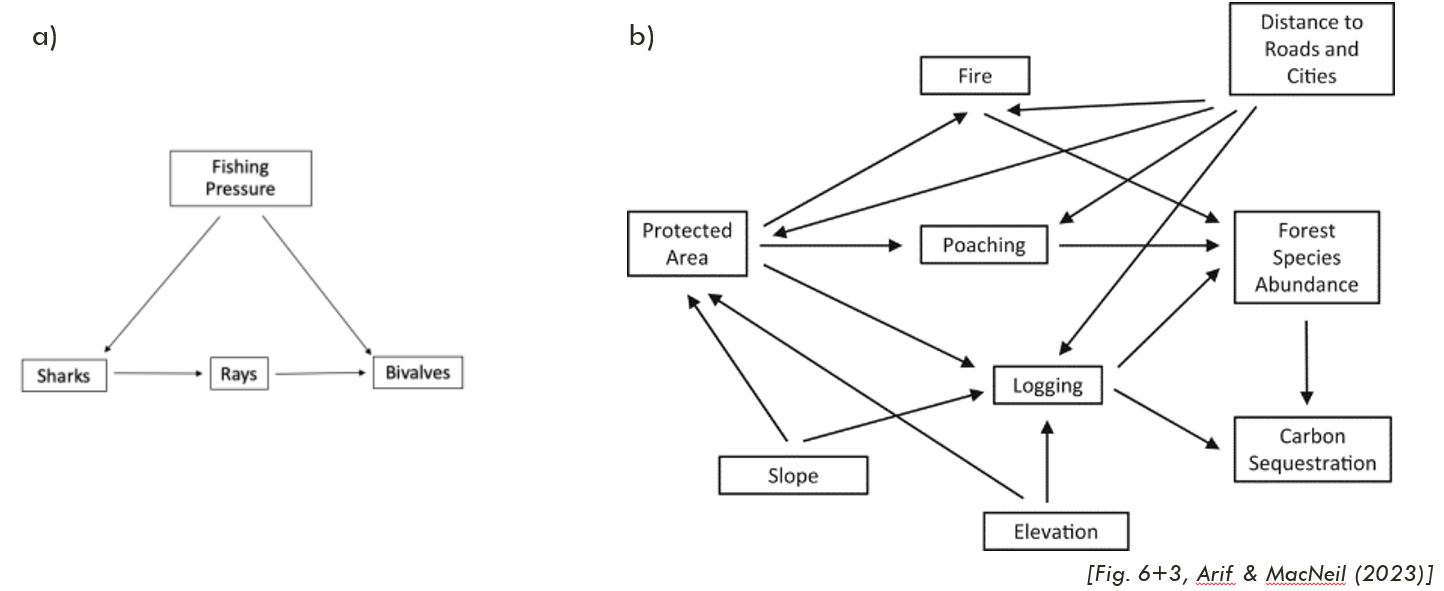
DAGs should include all causally relevant variables for the research question, including unmeasured ones. Depending on the purpose, DAGs can be quite simple as to highlight a specific relationship (Fig. 1a) or more comprehensive when reflecting a complex study system (Fig. 1b).

Importantly, a DAG is not a statistical model (e.g. GLM, SEM, GAM) and does not estimate effects. It is a conceptual tool that helps clarifying one’s a priori assumptions about causal relationships.

Two main purposes:

1) Helping you

• Display complex interactions
  A visual representation often makes it easier to understand a complex system. Identifying indirect pathways, missing or latent variables or potential lagged feedback structure will help to identify suitable analytical methods to correctly adressing the research question. In short: They help you make sense of your system

• Clarify the role of each variable
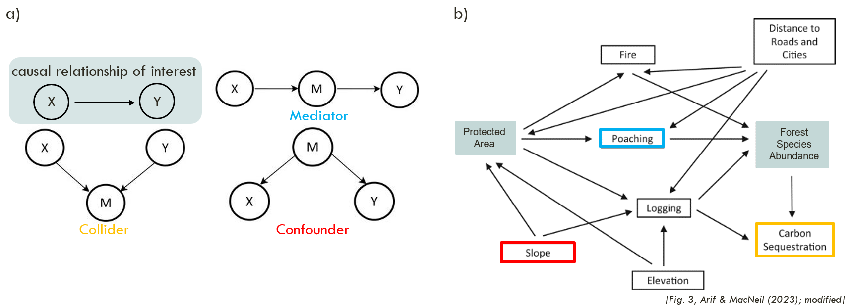
  The visual representation helps identify whether variables act as confounder, collider or mediator. The relevance depends on the estimand (e.g. total vs. direct effect): falsely omitting confounders or including colliders as covariates in a model will lead to biased estimates if the focus is on estimating an exposure’s total effect. Applying covariate adjustment helps identify the suitable minimal set of covariates, therefore can help to move from a ‘causal salad’ to thought-through effect estimation.

• Inform downstream model choice and implementation
  The causal structure clarified in a DAG can inform model specification. For example, by making unobserved confounders explicit it highlights which assumptions are strong and where effect estimation may fail. Covariate adjustment can help identify which variabes must be adjusted for. Importantly, the statistical model should reflect the causal model - not replace it.

2) Helping others (collegues, future readers…)

• Display complex interactions
  See above. What helps you structuring your thoughts about a system will even more facilitate the understanding among colleagues who are less familiar with your study system!

• Share (model) assumptions
  A DAG makes the underlying assumptions about a study system explicit. Which variables were considered? Which were omitted - on purpose or accidentally? This prevents post-hoc tweaking by making assumptions explicit beforehand. DAGs thus improve rigour and transparency, and (may) open and facilitate the scientific debate.

How to DAG:

Ideally, it is the first step of a project and proceeding any analysis. It can for example accompany the literature review in the beginning of the project, or the exchange with specialists. It further can (and should) be updated along when new findings appear.
To get started, you don’t need any tools; a blank paper or screen is enough. However, special tools (e.g. dagitty, R/Phyton libraries) can be useful as the DAG gets complex and overflowing.

While drawing, just keep in mind:

• Include all variables (you can always create a second, reduced version
  
• An arrow indicates a relationship between two variables, identifying exposure and outcome variable or bidirectionalilty but making no assumption about the form of that link (in next steps, you can of course add colors or labels to highlight shape of relationship or timelag).
  
• The absence of a link is meaningful!

In ecology, our DAGs will most often be expert DAGs, based on expert knowledge. In case no previous knowledge is available, causal discovery algorithms are available to infer plausible ‘causal’ structure from (time series) data itself (e.g. PCMCI, CCM). However, they come with strong assumptions (e.g. no hidden confounding, stationarity) and do not replace domain knowledge. Generally, the causal assumptions encoded in a DAG cannot be tested using

Covariate ajustment

Covariate adjustment, also back-door adjustment, is a basic, practical, method of causal inference aiming to remove confounding/biasing effects by identifying the appropriate set of variables to control for in a model (when estimating a ‘causal’ effect). The idea is to block non-causal pathways (i.e. backdor-pathways, those created by common causes/confounders) while keeping the causal pathway of interest open. In practice, this typically means adjusting for confounders (common causes of exposure and outcome). Mediators, which lie on the causal pathway, should not be adjusted for when estimating the total effect, as doing so blocks part of the effect of interest. Colliders, variables influenced by both exposure and outcome, should not be conditioned on, as this would open spurious associations and induce bias. The choice of covariates therefore is determined by the assumed causal structure and the specific estimand, not by statistical significance, automated model selection or simply availability of the data. It is possible, that for a given relationship of interest multiple (minimal) adjustment sets are possible. Tools such as DAGitty or R/Phyton libraries facilitate the identification of minimal adjustment set; Daggle provides some examples and exercises to get familiar with the backdoor-criteria.

Fig.2: a) Illustration of variable ‘M’ acting as mediator, collider or confounder in in the causal relationship between X and Y. b) identifies each type in a real world example. For example, when studying the total effect of ‘Protected Area’ on ‘Forest Species Abundance’, one would want to include ‘slope’ but omit ‘poaching’ and ‘carbon sequestration’ which might bias the estimation. Please note that these only are examples of confounder, mediator and collider in the displayed system (modified after Fig. 3 Arif & MacNeil (2023) )

Challenges

By definition, DAGs are ‘acyclic’. This can be challenging in ecology, where many systems show feedback loops. One way to overcome this is to use time-explicity DAGs which unfold the system over time (e.g. X_t -> Y_t+1 -> X_t+2) which preserves acyclicity while representign dynamic feedback. Another option is to focus on one time point, which should be explicitly stated.

Useful ressources

Lit

• Arif & MacNeil (2023) Applying the structural causal model framework for observational causal inference in ecology. Ecol Monographs vol 23 10.1002/ecm.1554
• Arif & MacNeil (2022) Predictive models aren’t for causal inference. Ecol. Letters vol 25 10.1111/ele.14033
• Borger & Ramesh (2023) Let’s DAG in: how directed acyclic graphs can help behavioural ecology be more transparent. Proc B vol 292 10.1098/rspb.2025.0963

Tools

• DAGitty.net (browser tool & R Package; draw DAG, determine role of covariates, identify (minimal) adjustment sets)
• dagR (R package to draw & identify (minimal) adjustment sets [less intuitive than DAGitty])
• DoWhy (Phython library; draw DAG, determine role of covariates, identify (minimal) adjustment sets)
• Daggle (a shiny app to learn and train the identification of minimal adjustment sets; links towards further beginner & advanced ressources)