The purpose of the package snakedist is to compute the
distance between each pair of locations by following the shape of a
curved line (e.g. a river).
Setup
# Custom ggplot2 theme ----
custom_theme <- function() {
  theme_light() +
  theme(plot.title   = element_text(face = "bold", family = "serif", size = 18),
        plot.caption = element_text(face = "italic", family = "serif"),
        axis.title   = element_blank(),
        axis.text    = element_text(family = "serif"))
}
Datasets
snakedist provides two datasets:
-
adour_lambert93: a spatial line layer (geopackage) of the French river L’Adour. -
adour_sites_coords: a table (csv) containing spatial coordinates of 5 locations sampled along the Adour.
First, let’s import the two datasets:
# Import the spatial layer of Adour river ----
path_to_file <- system.file("extdata", "adour_lambert93.gpkg",
                            package = "snakedist")
adour_river  <- sf::st_read(path_to_file, quiet = TRUE)
adour_river
#> Simple feature collection with 1 feature and 1 field
#> Geometry type: LINESTRING
#> Dimension:     XY
#> Bounding box:  xmin: 334324.8 ymin: 6207072 xmax: 480886.8 ymax: 6308530
#> Projected CRS: RGF93 v1 / Lambert-93
#>   river_name                           geom
#> 1    L'Adour LINESTRING (480886.8 620722...
# Import sites data ----
path_to_file <- system.file("extdata", "adour_sites_coords.csv",
                            package = "snakedist")
adour_sites  <- read.csv(path_to_file)
adour_sites
#>   site longitude latitude
#> 1 S-01  470911.2  6219515
#> 2 S-02  464962.6  6242684
#> 3 S-03  464023.4  6266791
#> 4 S-04  445238.4  6291838
#> 5 S-05  418626.3  6306239
The function distance_along() (main function of the
package) requires that both layers are spatial objects. So we need to
convert the data.frame adour_sites into an
sf object.
# Convert data.frame to sf object ----
adour_sites <- sf::st_as_sf(adour_sites, coords = c("longitude", "latitude"),
                            crs = "epsg:2154")
adour_sites
#> Simple feature collection with 5 features and 1 field
#> Geometry type: POINT
#> Dimension:     XY
#> Bounding box:  xmin: 418626.3 ymin: 6219515 xmax: 470911.2 ymax: 6306239
#> Projected CRS: RGF93 v1 / Lambert-93
#>   site                 geometry
#> 1 S-01 POINT (470911.2 6219515)
#> 2 S-02 POINT (464962.6 6242684)
#> 3 S-03 POINT (464023.4 6266791)
#> 4 S-04 POINT (445238.4 6291838)
#> 5 S-05 POINT (418626.3 6306239)
Let’s map the data.
# Visualize data ----
ggplot() +
  geom_sf(data = adour_river, col = "steelblue") +
  geom_sf(data = adour_sites, shape = 19, size = 2) +
  geom_sf_label(data = adour_sites, aes(label = site), nudge_x = 5000) +
  geom_text(aes(x = 334500, y = 6285000), label = "L'Adour", hjust = 0,
            color = "steelblue", fontface = "bold", size = 6, family = "serif") +
  labs(caption = "RGF93 / Lambert-93 Projection") +
  custom_theme()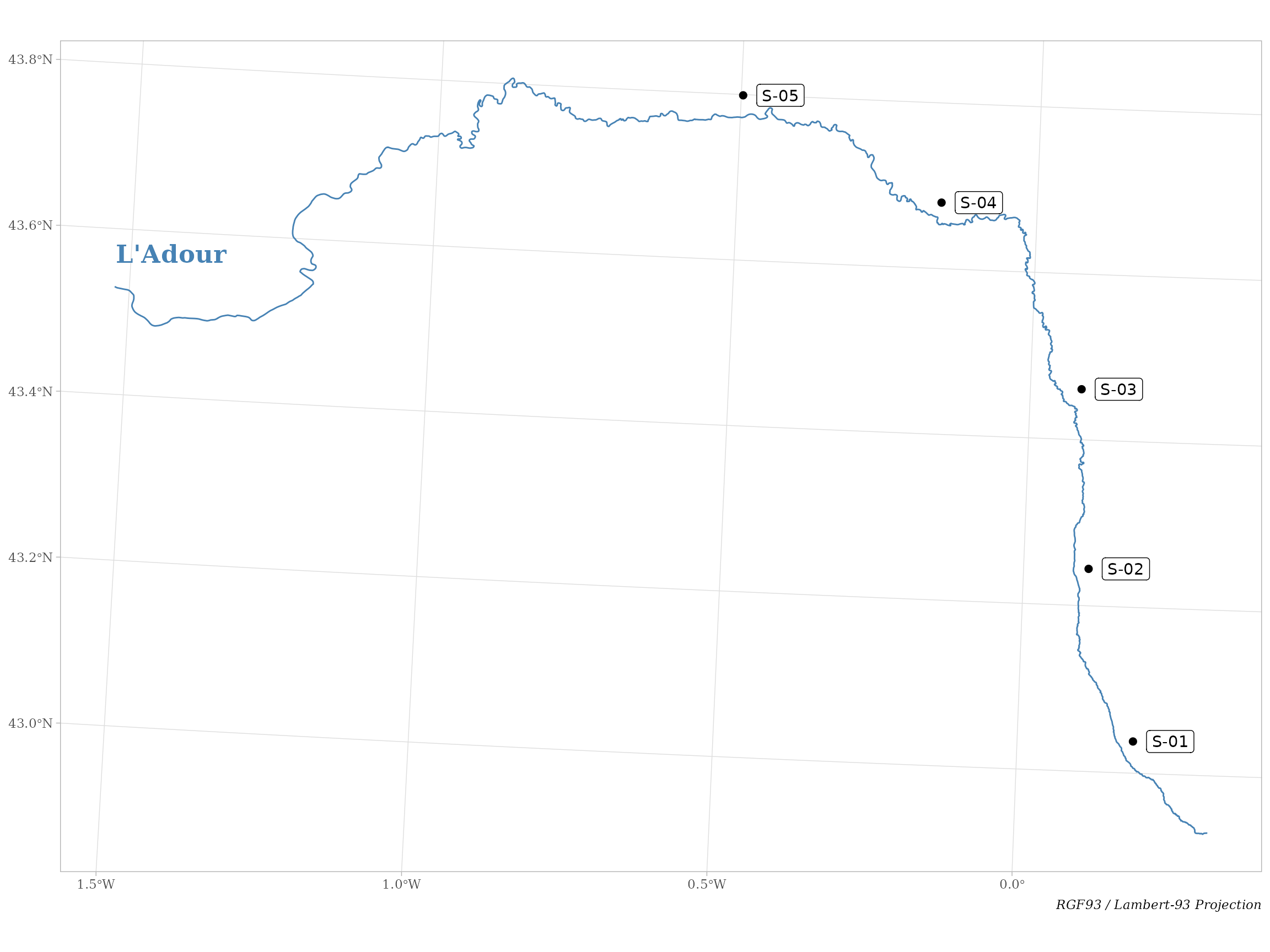
Figure 1. Study area with survey sampling
Compute distances
The function distance_along() computes the distance
between pairs of sites by following the shape of a linear structure (in
our case the river Adour). It uses the function
sf::st_line_sample() to regularly (or randomly, argument
type) sample points on the line with a given density of
points (argument density). All sampled points between the
two sites will be selected and their cumulative euclidean distance will
be computed.
# Compute distance along the river ----
dists <- distance_along(adour_sites, adour_river, density = 0.01, type = "regular")
head(dists, 12)
#> from to distance
#> 1 S-01 S-01 0.00
#> 2 S-01 S-02 27422.59
#> 3 S-01 S-03 52913.17
#> 4 S-01 S-04 103064.90
#> 5 S-01 S-05 144881.86
#> 6 S-02 S-01 27422.59
#> 7 S-02 S-02 0.00
#> 8 S-02 S-03 25490.58
#> 9 S-02 S-04 75642.30
#> 10 S-02 S-05 117459.27
#> 11 S-03 S-01 52913.17
#> 12 S-03 S-02 25490.58This data.frame can be converted to a square matrix with
the function df_to_matrix().
# Convert to square matrix ----
df_to_matrix(dists)
#>           S-01      S-02     S-03      S-04      S-05
#> S-01      0.00  27422.59 52913.17 103064.90 144881.86
#> S-02  27422.59      0.00 25490.58  75642.30 117459.27
#> S-03  52913.17  25490.58     0.00  50151.72  91968.69
#> S-04 103064.90  75642.30 50151.72      0.00  41816.97
#> S-05 144881.86 117459.27 91968.69  41816.97      0.00
We can compare these values with the Euclidean distance.
# Compare to Euclidean distance ----
coords <- sf::st_coordinates(adour_sites)
dist(coords, upper = TRUE, diag = TRUE)
#>           1         2         3         4         5
#> 1      0.00  23919.63  47774.67  76743.68 101265.81
#> 2  23919.63      0.00  24125.69  52963.81  78653.68
#> 3  47774.67  24125.69      0.00  31308.31  60142.11
#> 4  76743.68  52963.81  31308.31      0.00  30259.12
#> 5 101265.81  78653.68  60142.11  30259.12      0.00
This package is related to the package chessboard.