This function applies a Bayesian model to count series in order to infer
the population trend over time. This function only works on the output of
format_data() or filter_series().
Important: This function uses R2jags::jags() and the
freeware JAGS (https://mcmc-jags.sourceforge.io/) must be
installed.
There are two types of options: model options (argument model_opts) and
MCMC options (argument mcmc_opts).
A. Model options
a smoothing factor: the precision (the inverse of variance) of a normal distribution centered on the current relative rate of increase r from which the next candidate relative rate of increase (see below) is drawn. The highest this number, the tighter the link between successive relative rates of increase. The default
100corresponds to a moderate link.a logical indicating whether the population growth must remain limited by the species demographic potential (provided by the argument
rmaxinformat_data()).
The relative rate of increase is the change in log population size between two dates. The quantity actually being modeled is the relative rate of increase per unit of time (usually one date). This quantity reflects more directly the prevailing conditions than the population size itself, which is the reason why it has been chosen.
When the second model option is set to TRUE, the candidate rate of
increase is compared to the maximum relative rate of increase
(obtained when using format_data()) and replaced by rmax if greater.
B. MCMC options
Classical Markov chain Monte Carlo (MCMC) settings (see argument mcmc_opts
below).
Arguments
- data
a named
list. The output offormat_data()orfilter_series().- model_opts
a
listof two vectors. The model smoothing factor (numeric) and alogicalindicating if the parameter r must be limited byrmax(TRUE) or not (FALSE). If this second parameter isTRUE, the argumentrmaxcannot beNULLunless species are listed inpopbayes(inspecies_info).- mcmc_opts
a
listcontaining the number of iterations (ni), the thinning factor (nt), the length of burn in (nb), i.e. the number of iterations to discard at the beginning, and the number of chains (nc).- path
a
characterstring. The directory to save BUGS outputs (the same as informat_data()).
Value
An n-element list (where n is the number of count series). Each
element of the list is a BUGS output as provided by JAGS (also written
in the folder path).
Examples
## Load Garamba raw dataset ----
file_path <- system.file("extdata", "garamba_survey.csv",
package = "popbayes")
garamba <- read.csv(file = file_path)
## Create temporary folder ----
temp_path <- tempdir()
## Format dataset ----
garamba_formatted <- popbayes::format_data(
data = garamba,
path = temp_path,
field_method = "field_method",
pref_field_method = "pref_field_method",
conversion_A2G = "conversion_A2G",
rmax = "rmax")
#> ✔ Detecting 10 count series.
## Get data for Alcelaphus buselaphus at Garamba only ----
a_buselaphus <- popbayes::filter_series(garamba_formatted,
location = "Garamba",
species = "Alcelaphus buselaphus")
#> ✔ Found 1 series with "Alcelaphus buselaphus" and "Garamba".
# \donttest{
## Fit population trend (requires JAGS) ----
a_buselaphus_mod <- popbayes::fit_trend(a_buselaphus, path = temp_path)
#> Compiling data graph
#> Resolving undeclared variables
#> Allocating nodes
#> Initializing
#> Reading data back into data table
#> Compiling model graph
#> Resolving undeclared variables
#> Allocating nodes
#> Graph information:
#> Observed stochastic nodes: 15
#> Unobserved stochastic nodes: 15
#> Total graph size: 227
#>
#> Initializing model
#>
## Check for convergence ----
popbayes::diagnostic(a_buselaphus_mod, threshold = 1.1)
#> ✔ All models have converged.
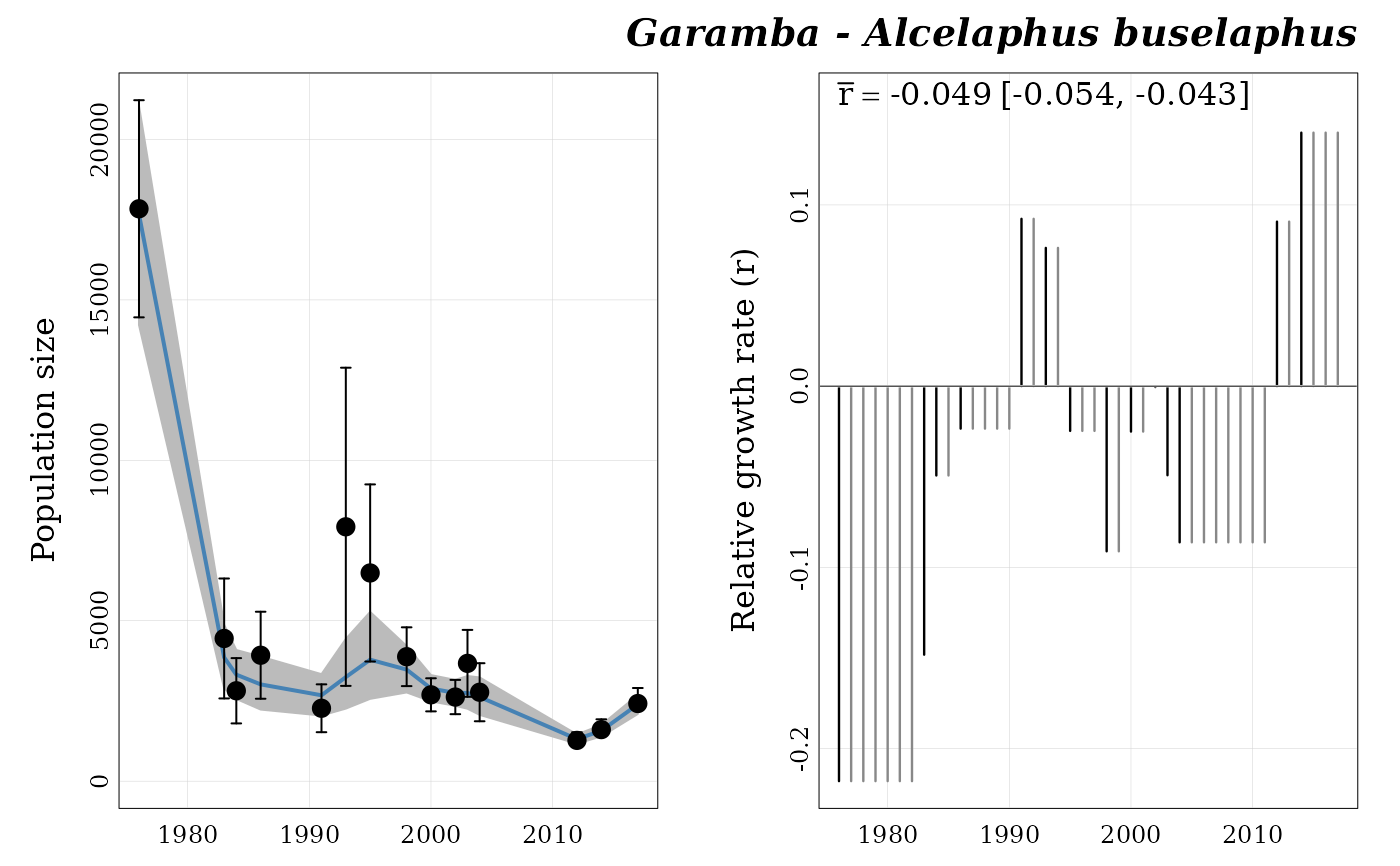
## Plot estimated population trend ----
popbayes::plot_trend(series = "garamba__alcelaphus_buselaphus",
path = temp_path)
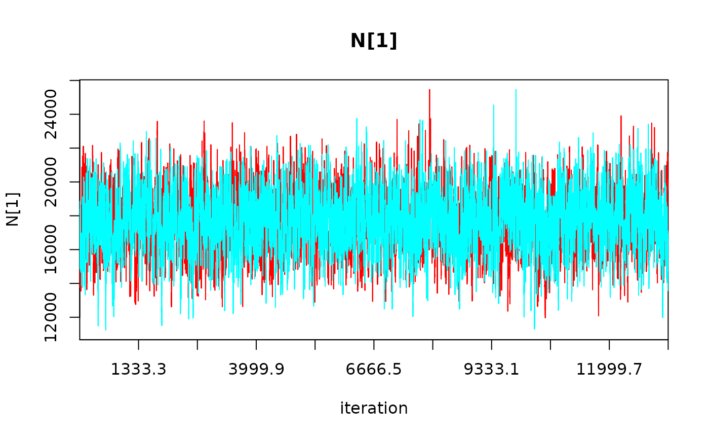
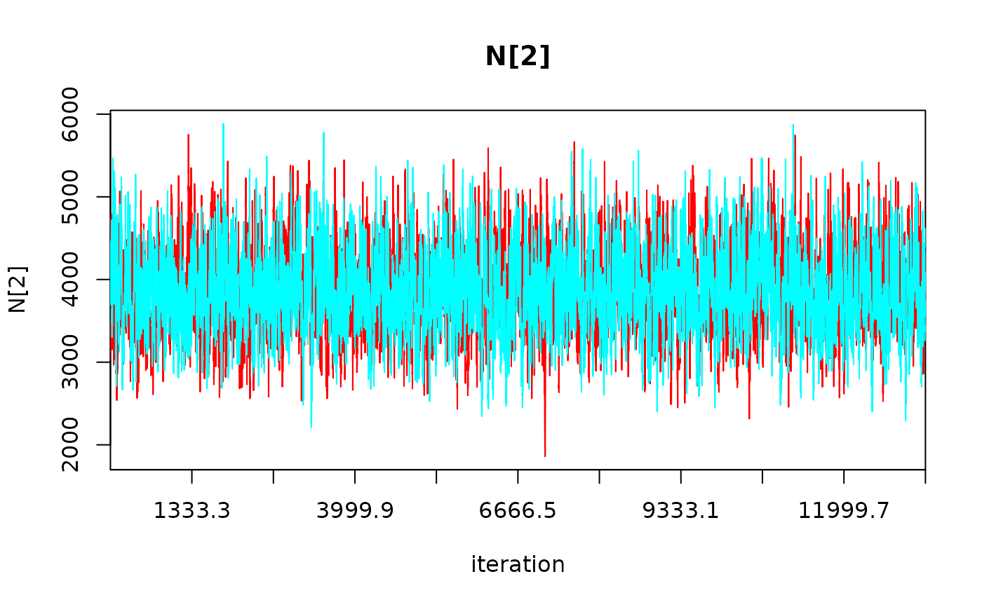
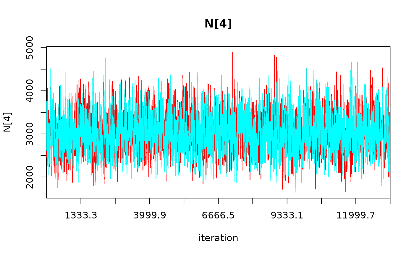
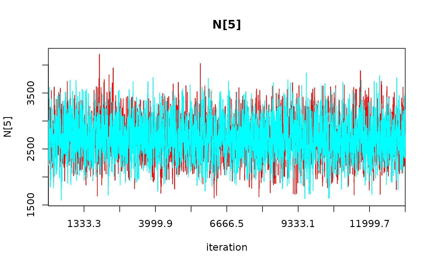
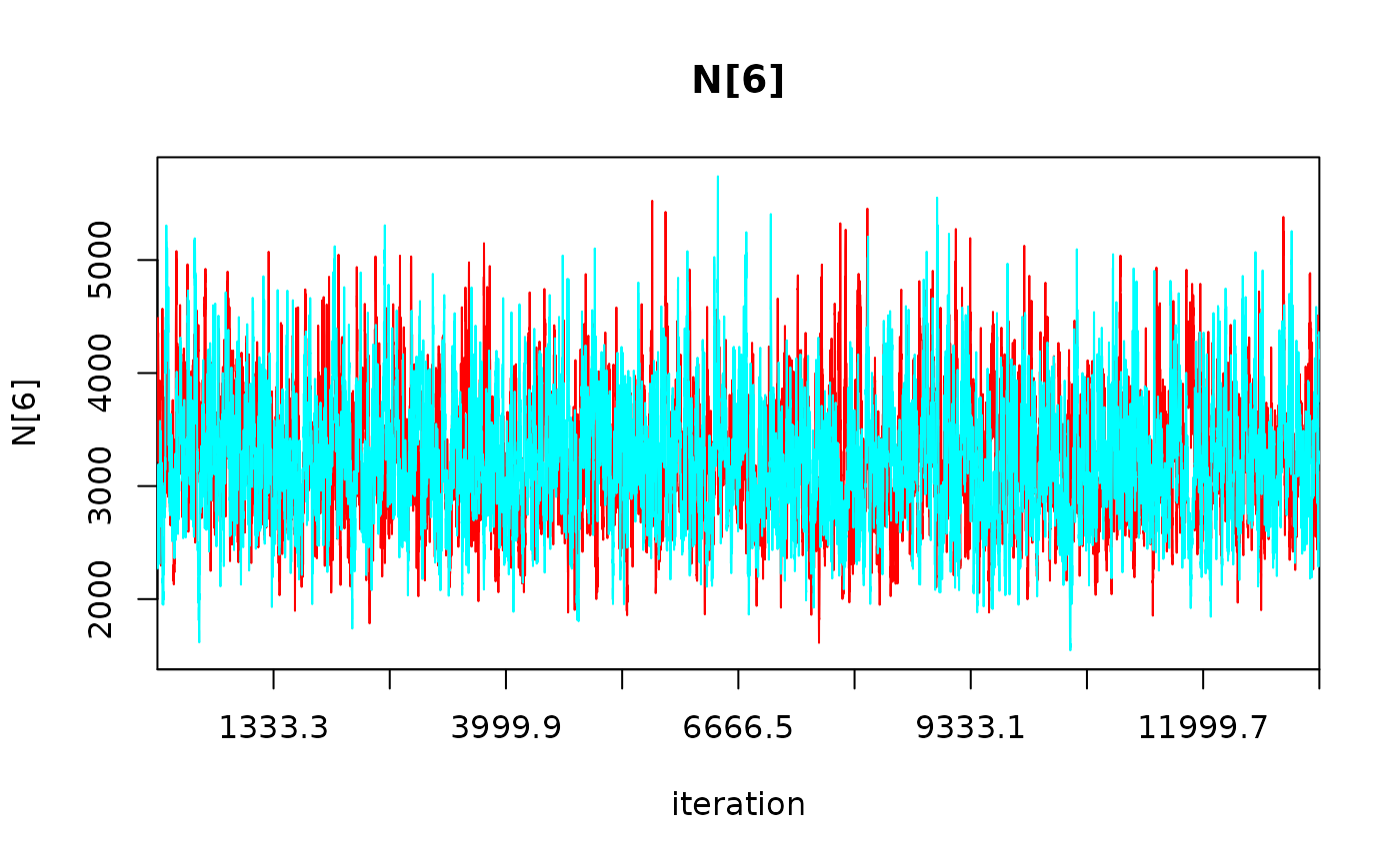
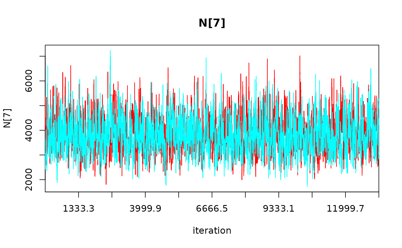
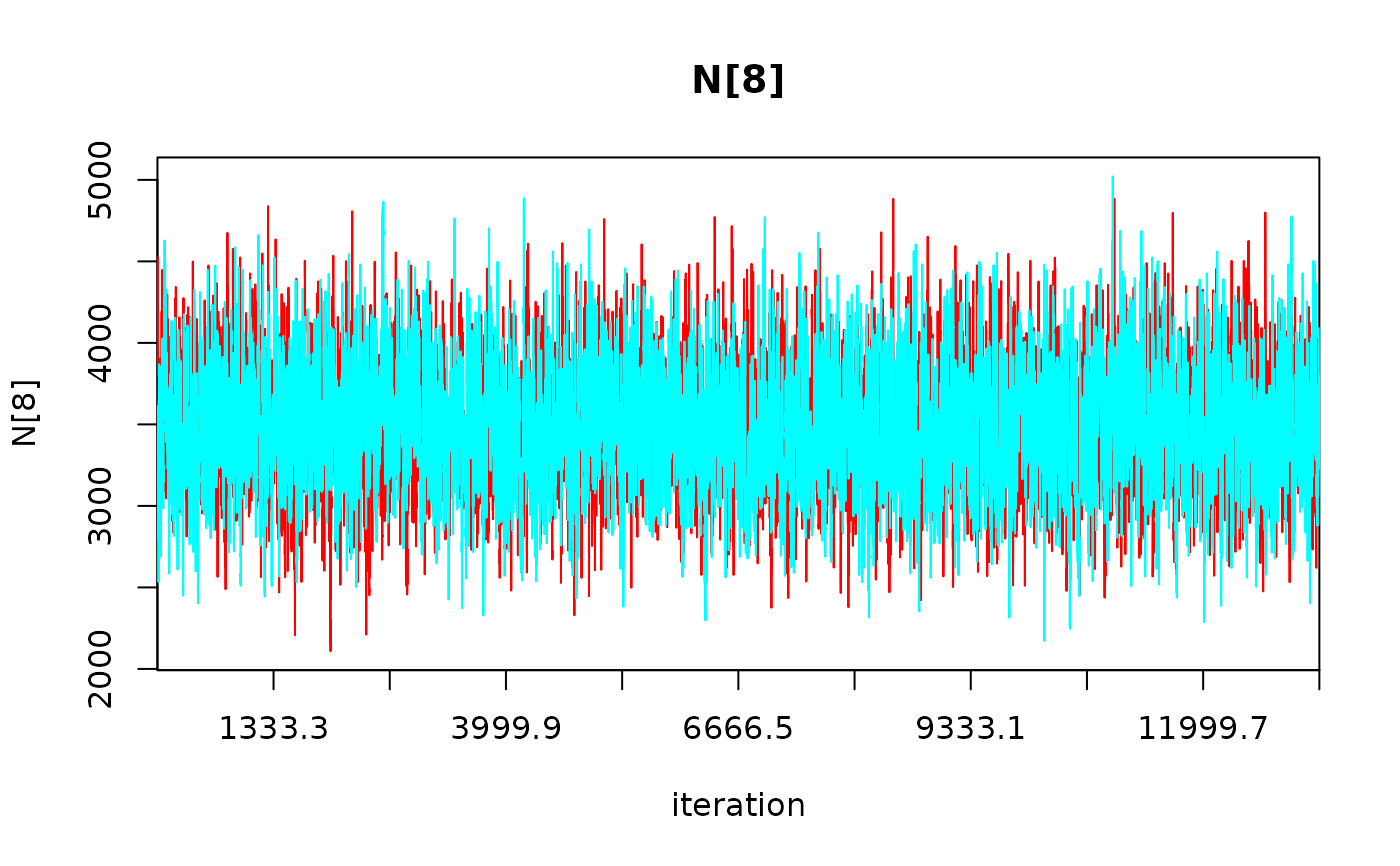
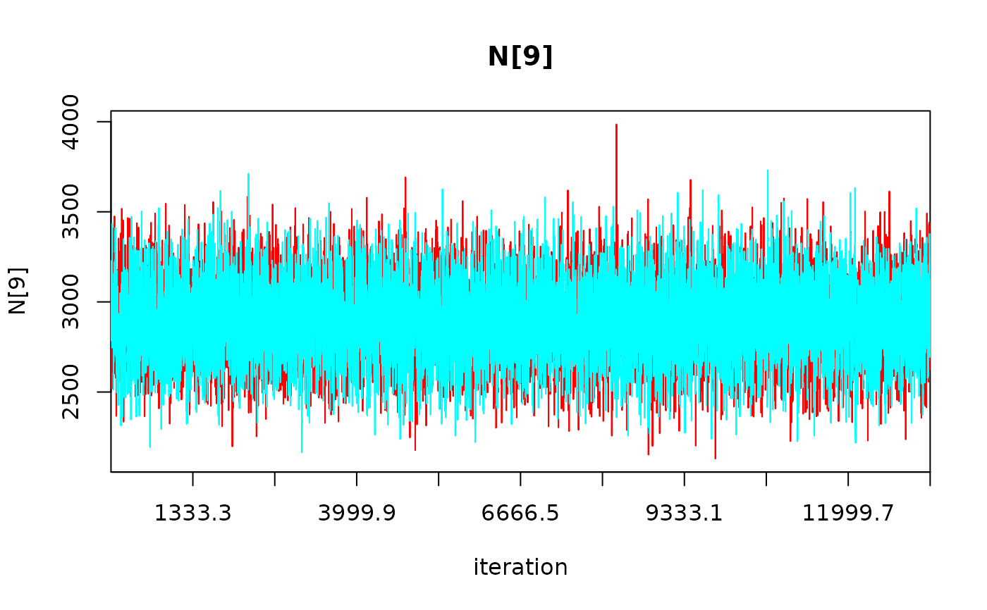
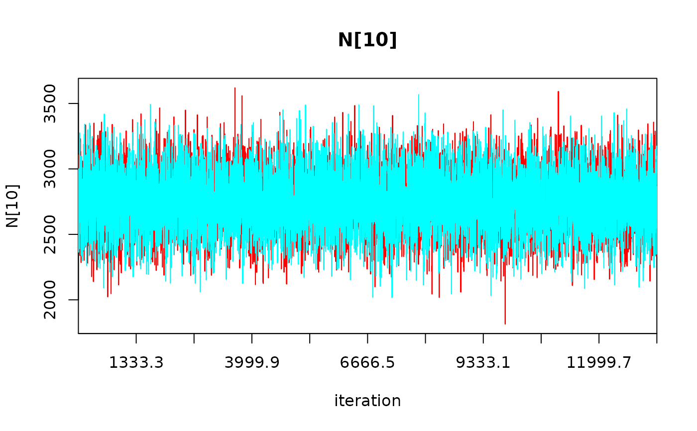
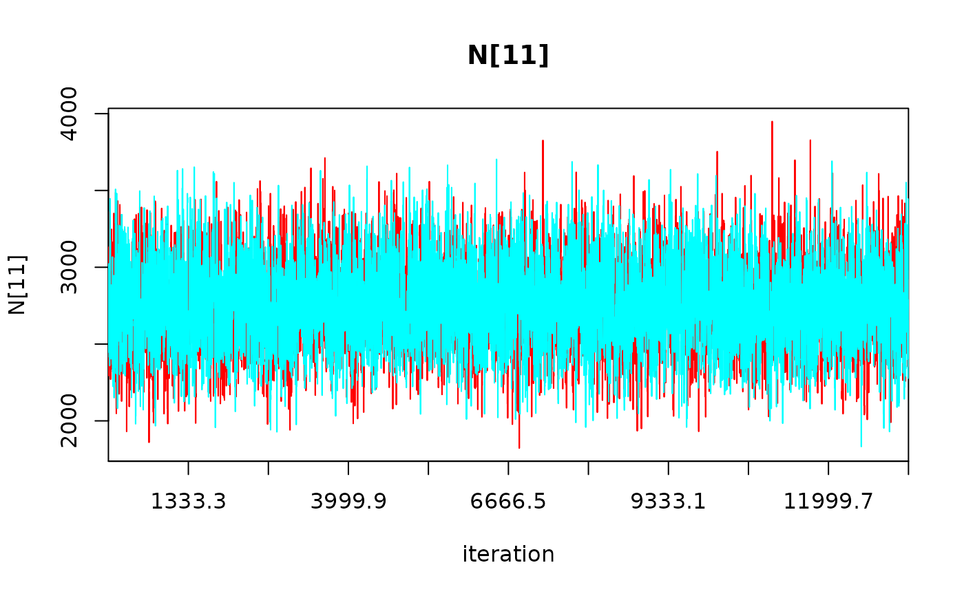
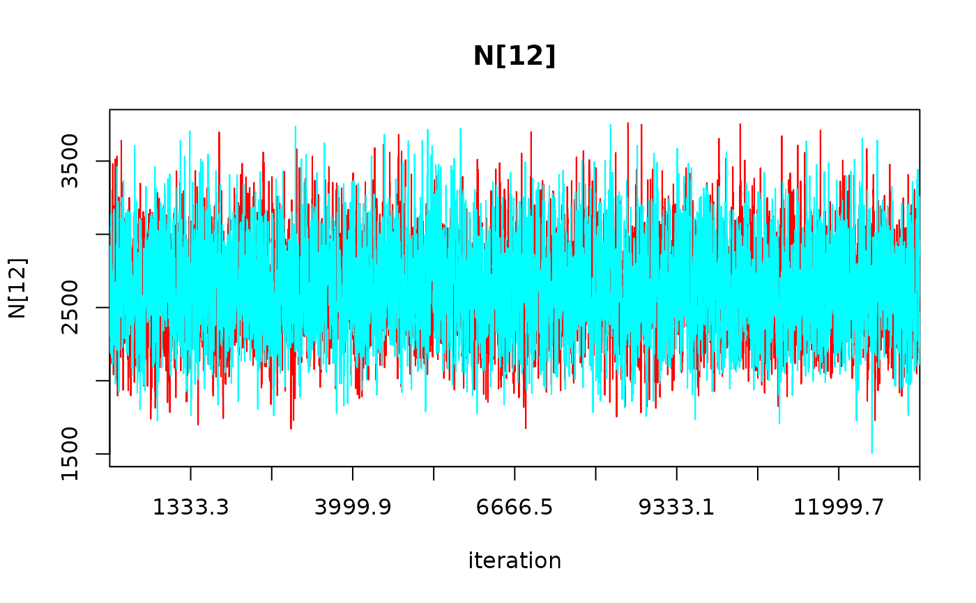
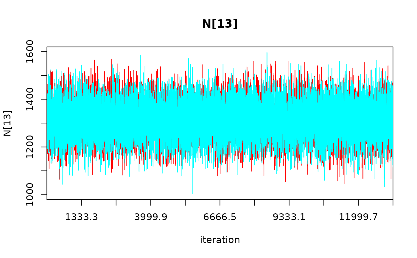
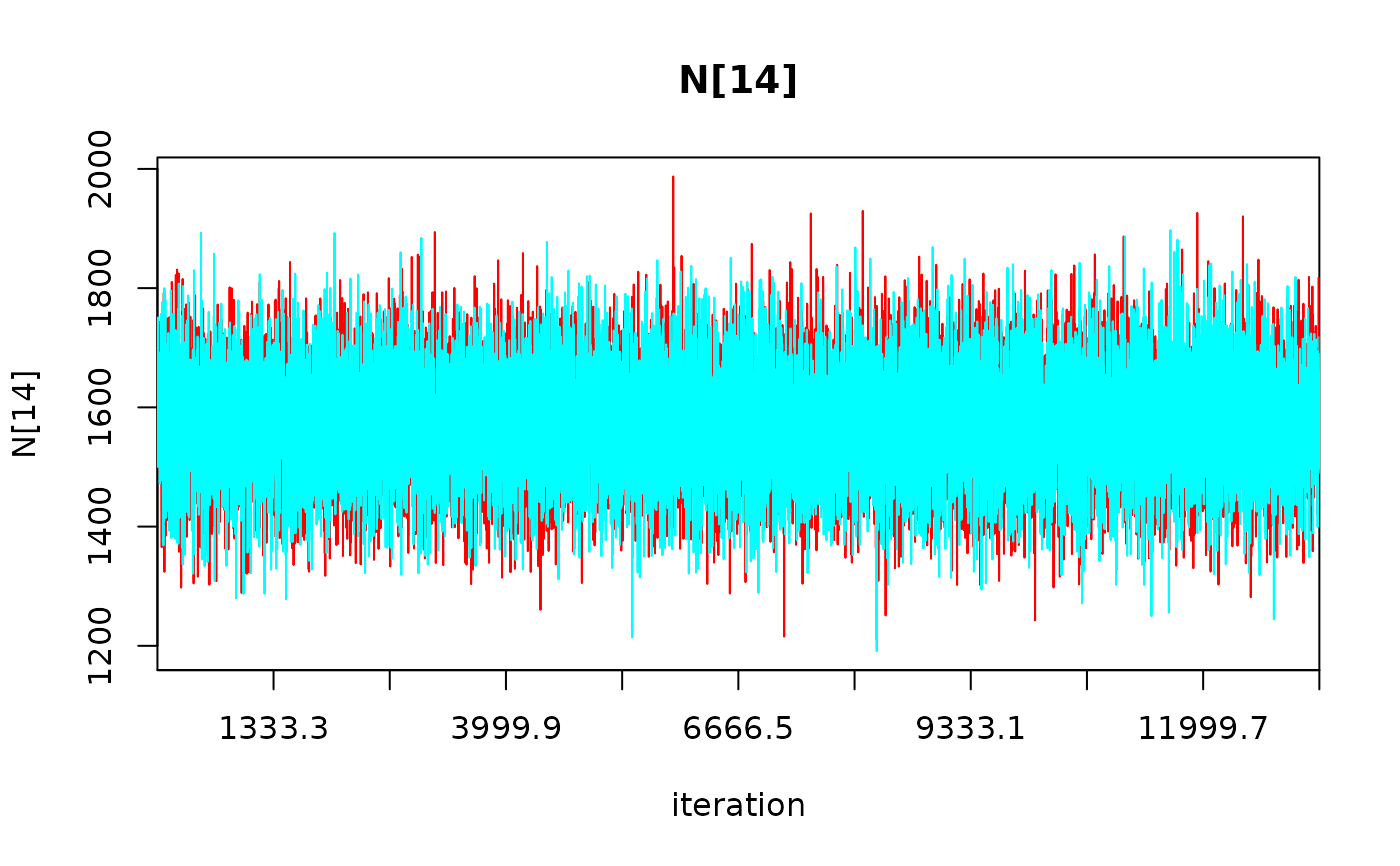
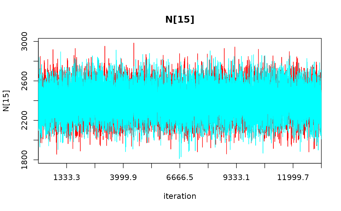
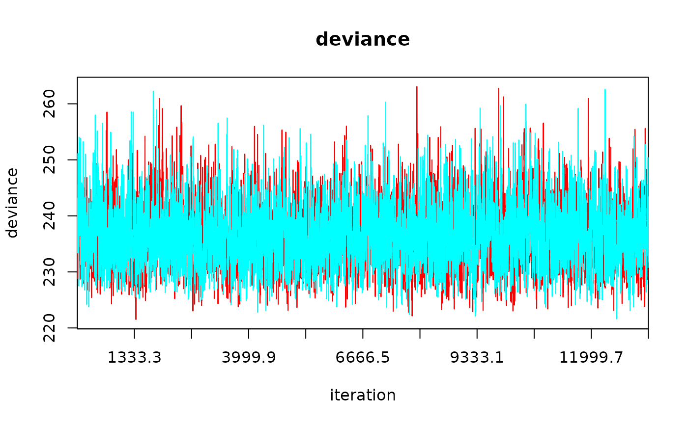
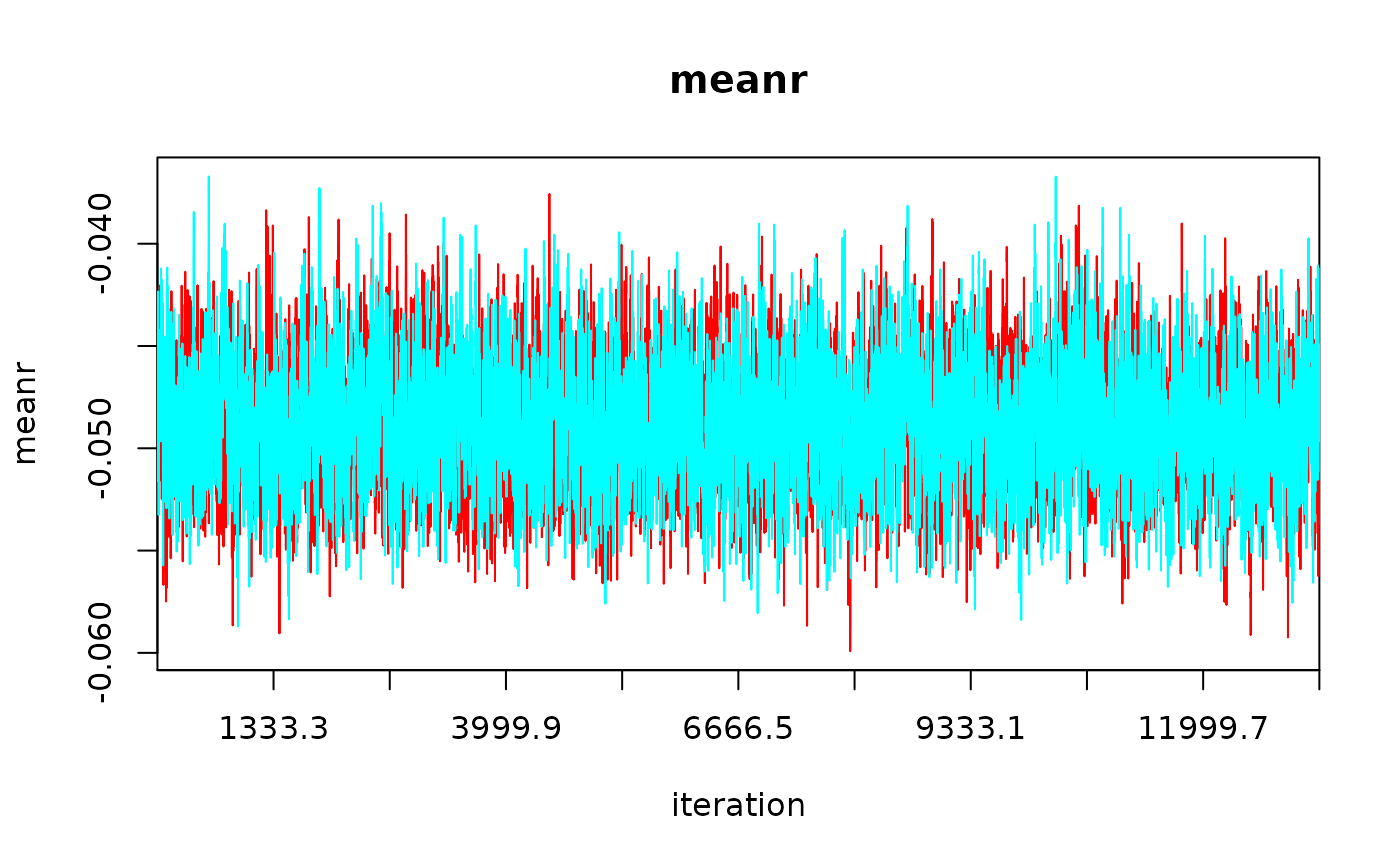
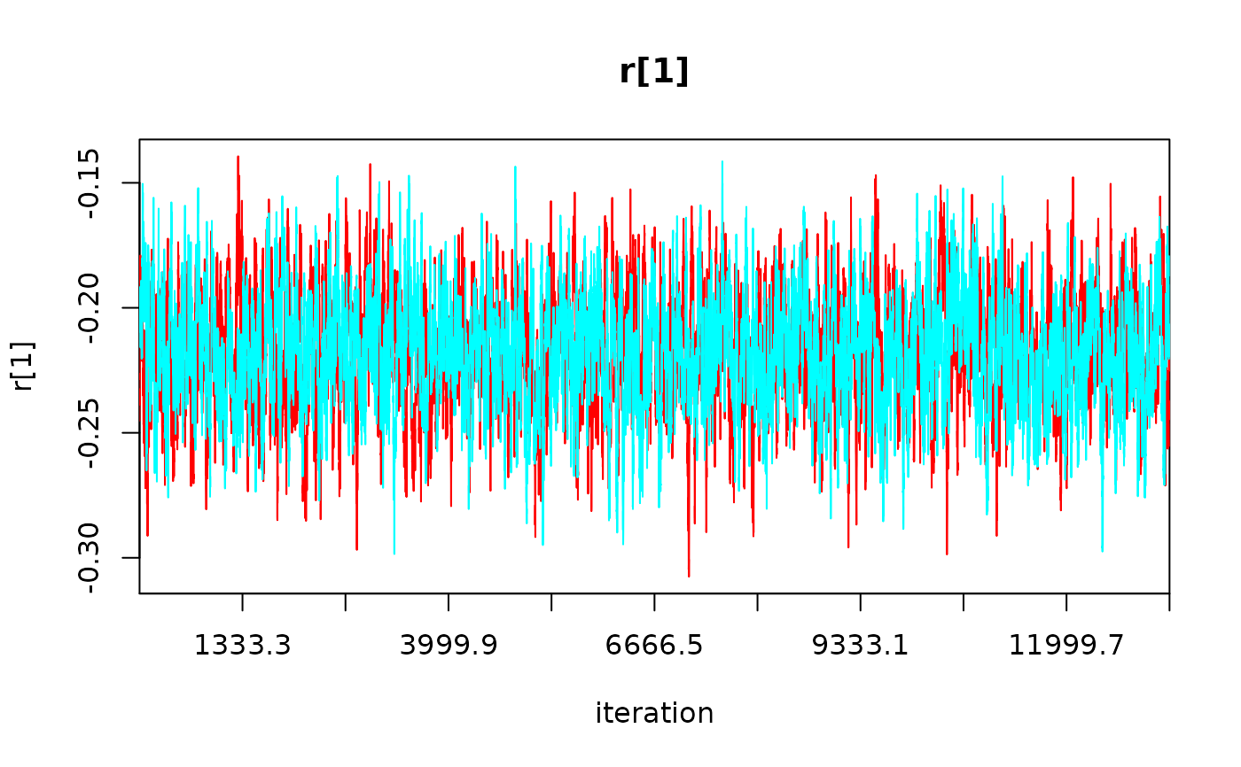
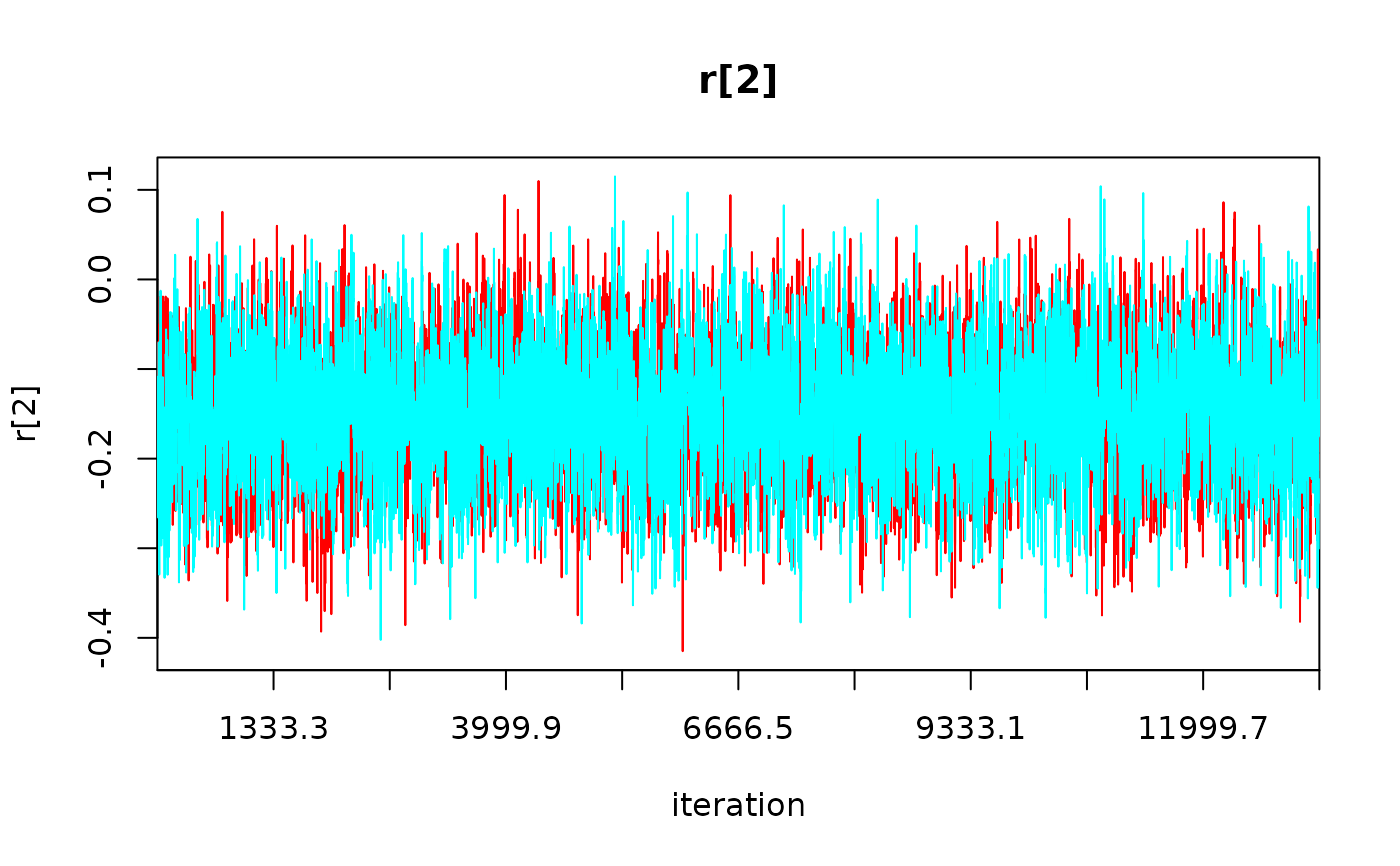
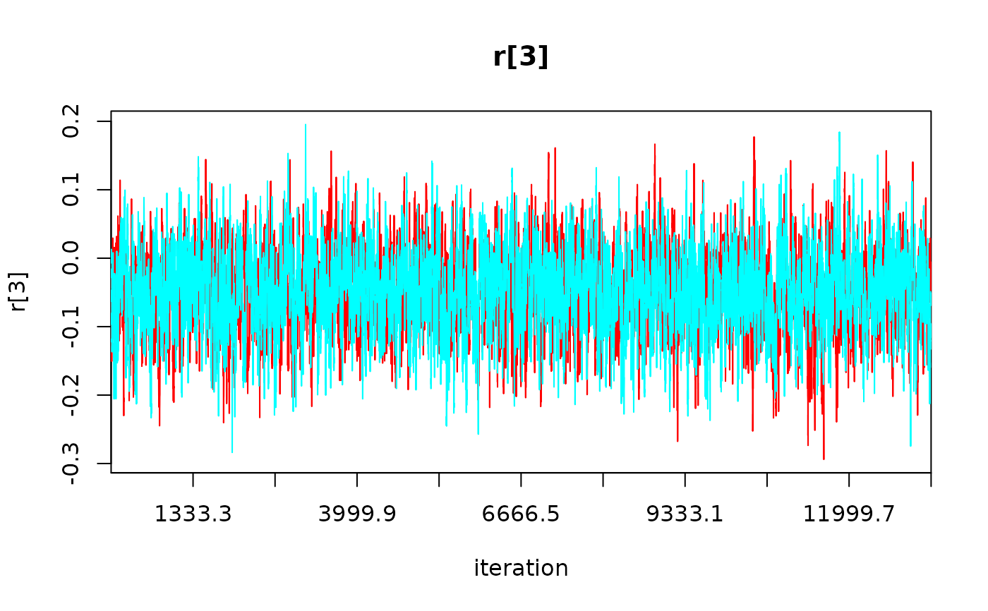
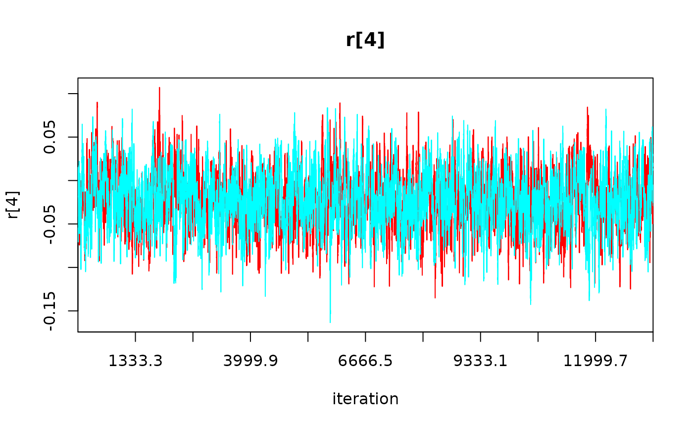
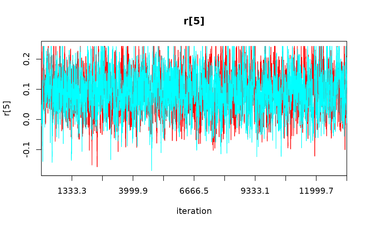
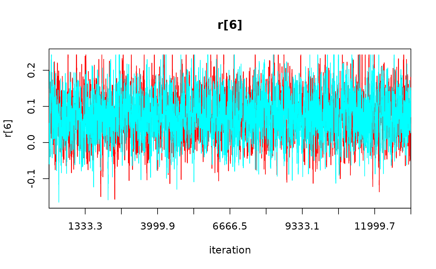
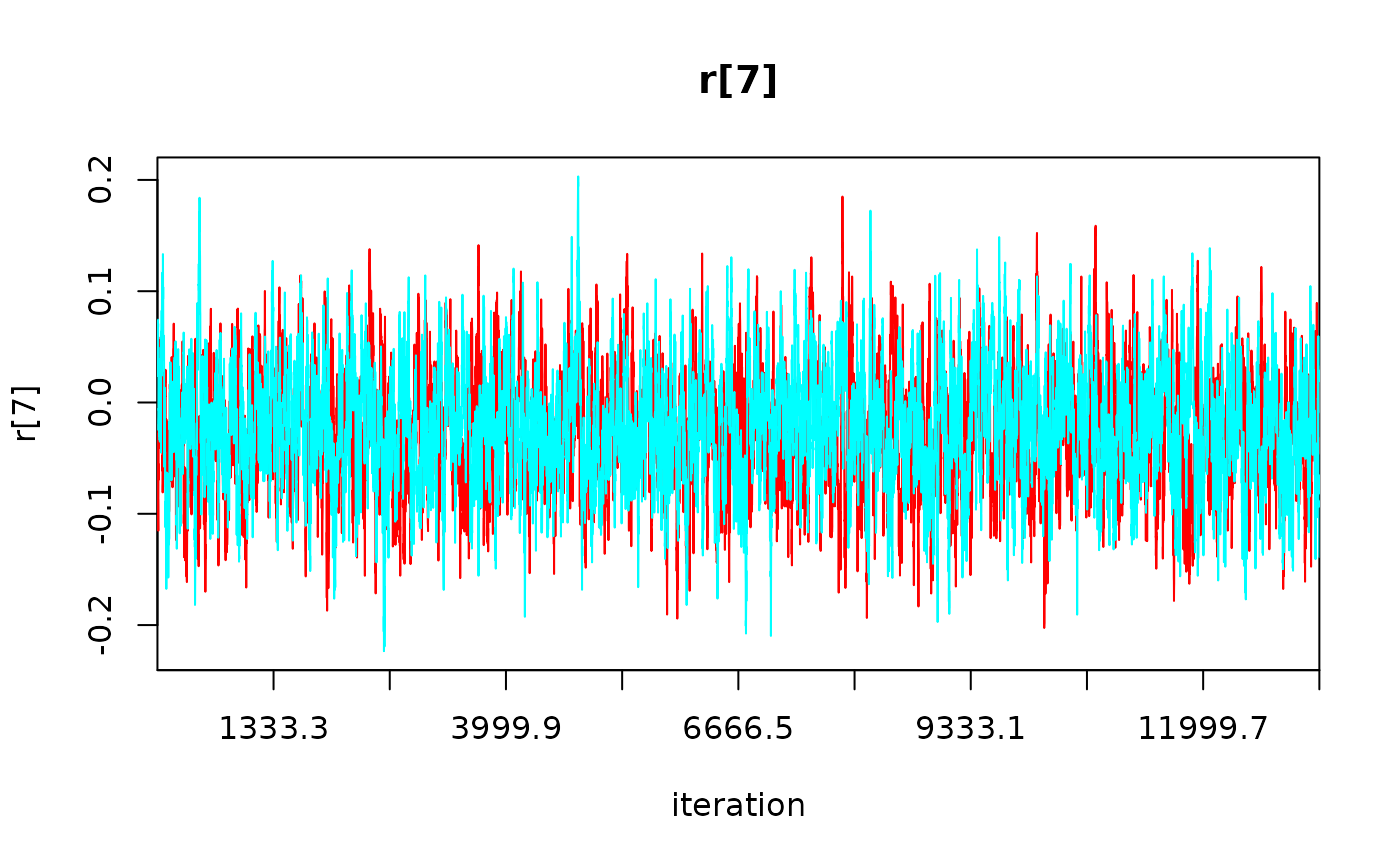
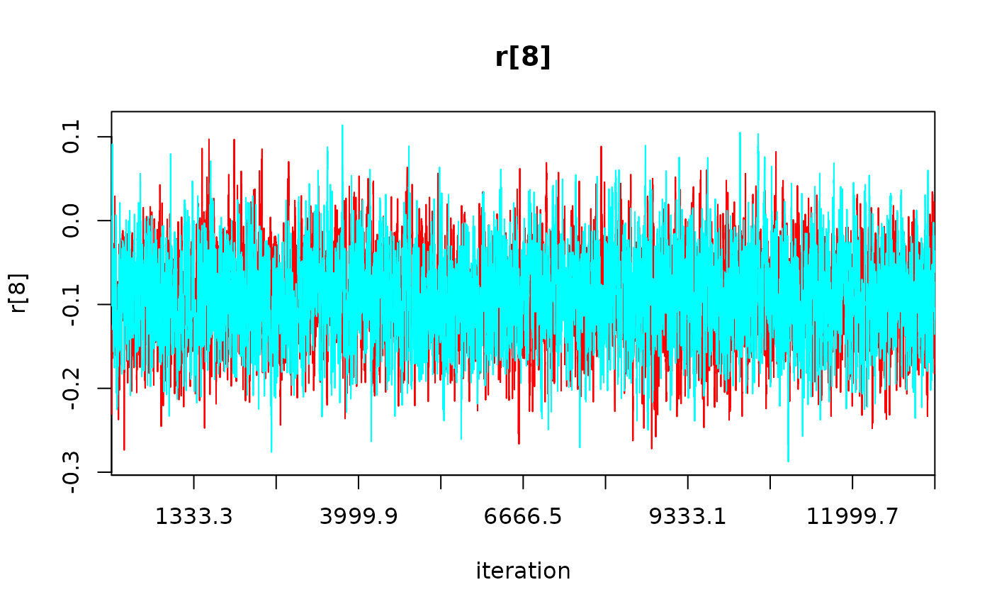
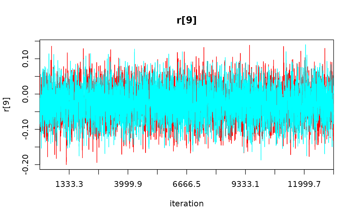
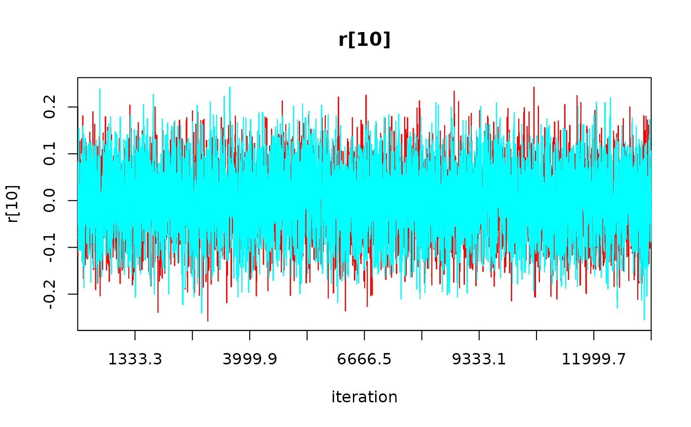
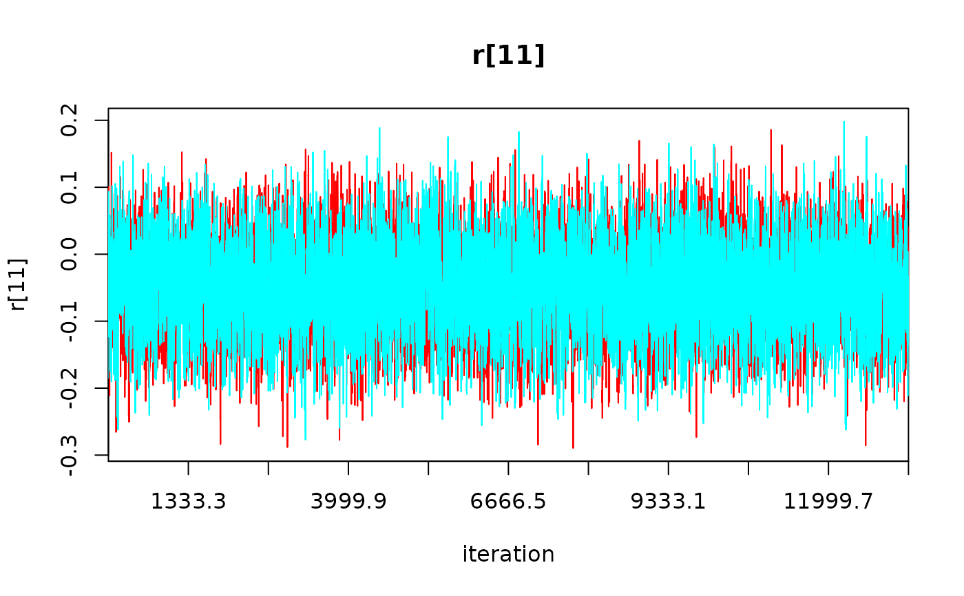
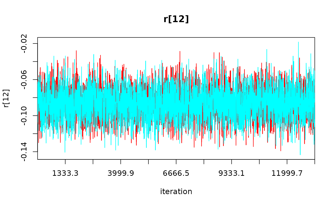
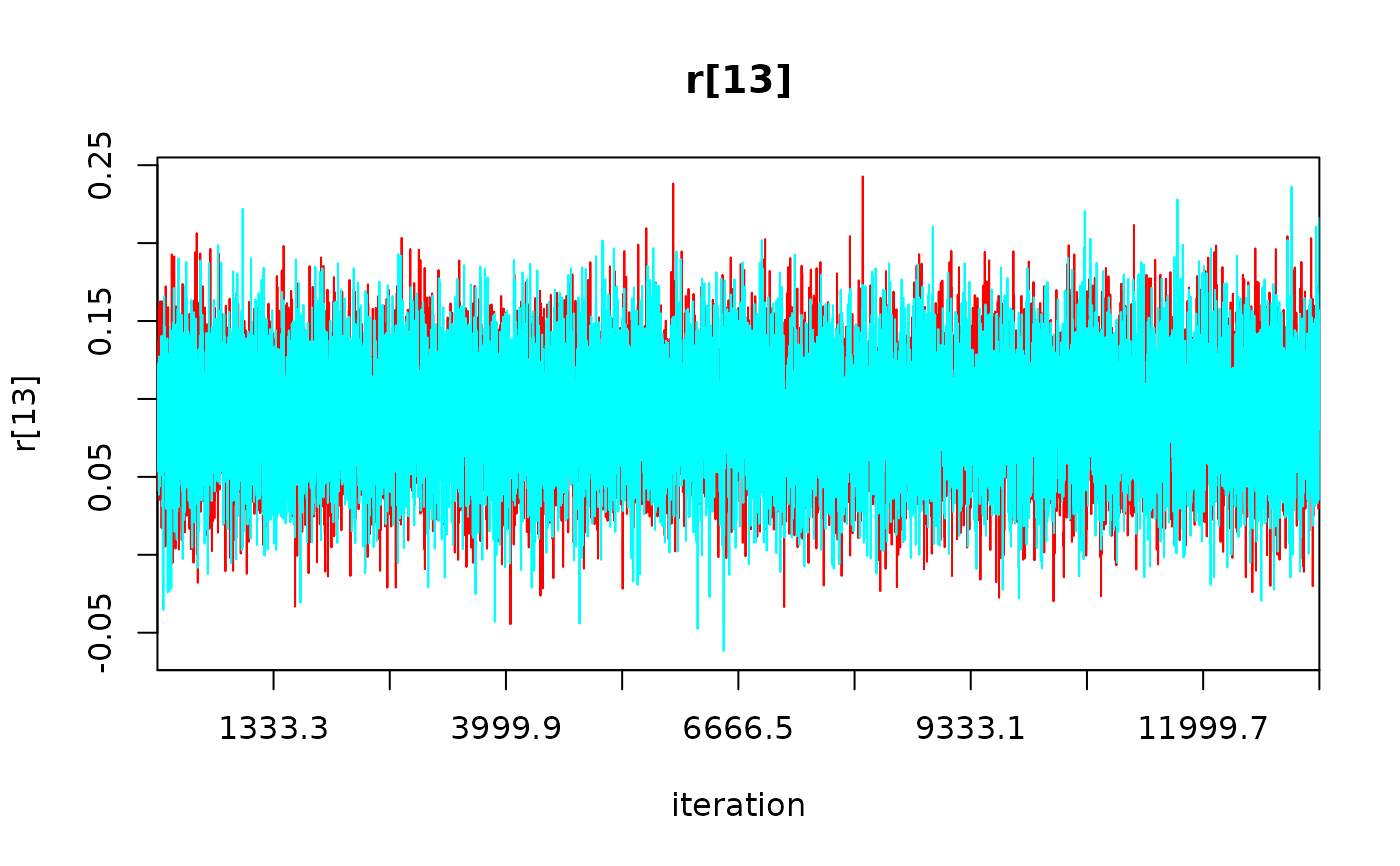
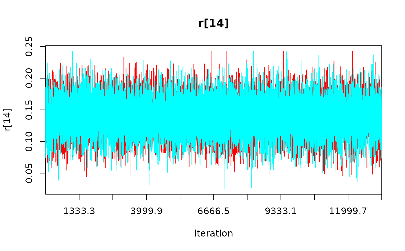
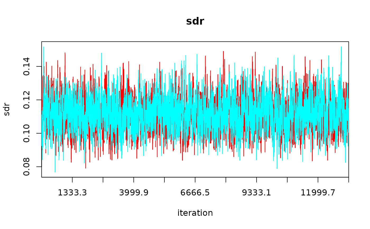
 ## Plot MCMC traceplot ----
R2jags::traceplot(a_buselaphus_mod[[1]], ask = TRUE)
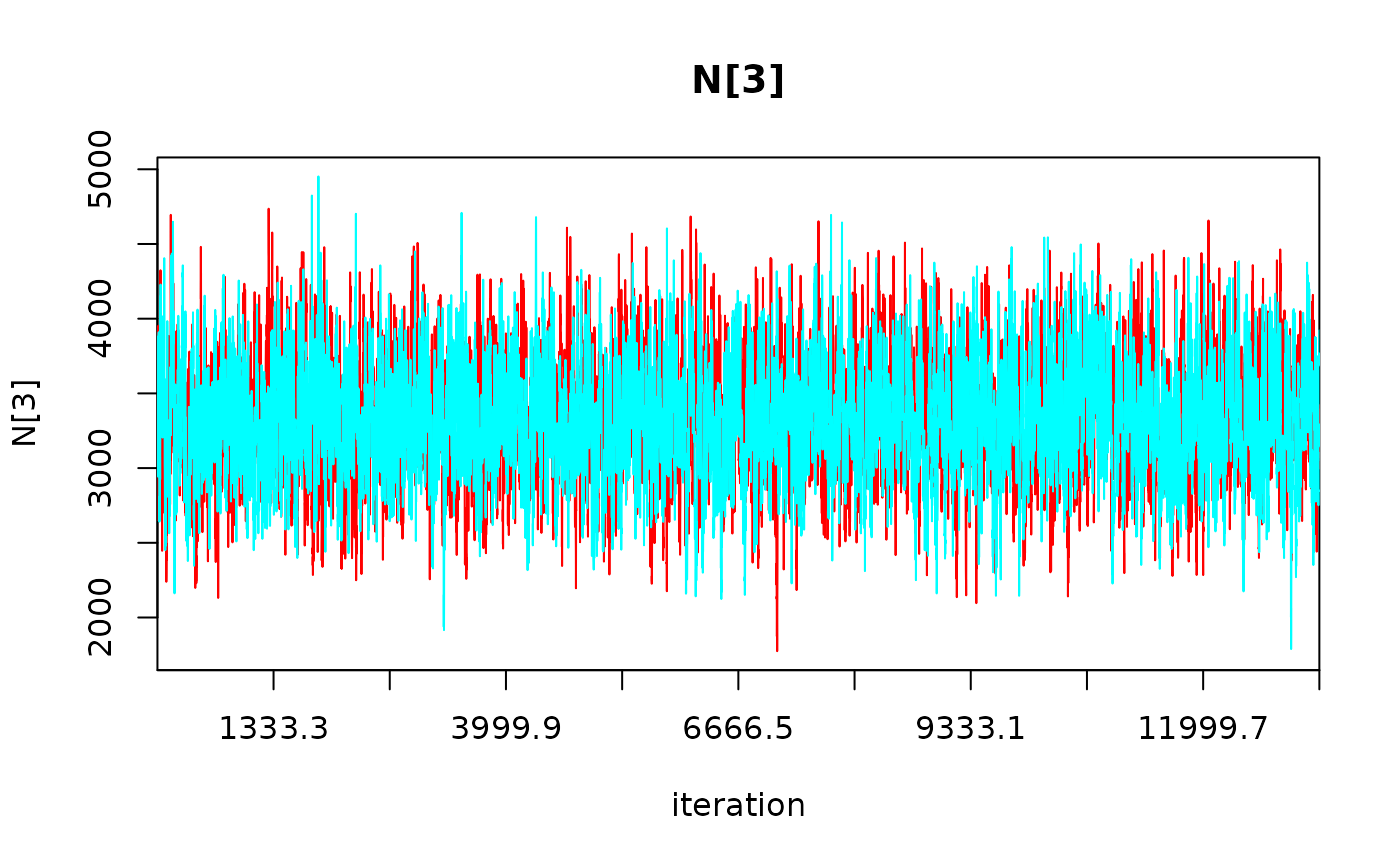
## Plot MCMC traceplot ----
R2jags::traceplot(a_buselaphus_mod[[1]], ask = TRUE)
 # }
# }