Plot estimated population trend — plot

This function plots a panel of two graphics for one BUGS model (previously generated by fit_trend()):

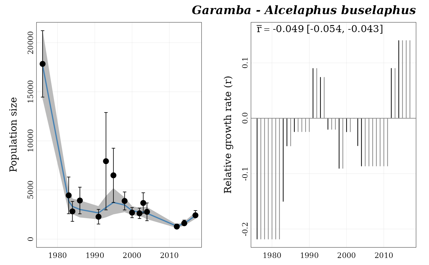
on the left side, the population trend estimated by the Bayesian model (blue line) with the 95% CI (gray envelop). Dots (with intervals) represent converted counts passed to the model (with the 95% CI);
on the right side, a bar plot of estimated relative growth rates (r) by date. Dark bars are real estimated r.

Usage

plot_trend(series, title = TRUE, path = ".", path_fig = ".", save = FALSE)

Arguments

series: a character string. The count series name (can be retrieved by running list_series()).
title: a logical. If TRUE (default) a title (series name) is added.
path: a character string. The directory in which count series (and BUGS outputs) have been saved by the function format_data() (and by fit_trend()).
path_fig: a character string. The directory where to save the plot (if save = TRUE). This directory must exist and can be an absolute or a relative path.
save: a logical. If TRUE (default is FALSE) the plot is saved in path_fig.

Value

No return value.

Examples

## Load Garamba raw dataset ----
file_path <- system.file("extdata", "garamba_survey.csv", 
                         package = "popbayes")
                         
garamba <- read.csv(file = file_path)

## Create temporary folder ----
temp_path <- tempdir()

## Format dataset ----
garamba_formatted <- popbayes::format_data(
  data              = garamba, 
  path              = temp_path,
  field_method      = "field_method",
  pref_field_method = "pref_field_method",
  conversion_A2G    = "conversion_A2G",
  rmax              = "rmax")
#> ✔ Detecting 10 count series.

## Select one serie ----
a_buselaphus <- popbayes::filter_series(garamba_formatted, 
                                        location = "Garamba",
                                        species  = "Alcelaphus buselaphus")
#> ✔ Found 1 series with "Alcelaphus buselaphus" and "Garamba".
# \donttest{
## Fit population trends (requires JAGS) ----
a_buselaphus_mod <- popbayes::fit_trend(a_buselaphus, path = temp_path)
#> Compiling data graph
#>    Resolving undeclared variables
#>    Allocating nodes
#>    Initializing
#>    Reading data back into data table
#> Compiling model graph
#>    Resolving undeclared variables
#>    Allocating nodes
#> Graph information:
#>    Observed stochastic nodes: 15
#>    Unobserved stochastic nodes: 15
#>    Total graph size: 227
#> 
#> Initializing model
#> 

## Plot estimated population trend ----
popbayes::plot_trend(series = "garamba__alcelaphus_buselaphus", 
                     path   = temp_path)

# }