About

This tutorial describes the basic workflow showing how to compute step by step functional diversity (FD) indices in a multidimensional space. It is divided in three parts:

Computing trait-based distances and the multidimensional functional space
Using the mFD package to compute FD alpha and beta indices and plot them (Magneville et al. 2021)
Using the funrar package to compute functional rarity indices (Violle et al. 2017, Grenié et al. 2017)

N.B. You can chose to do Part 2 and Part 3 in the order that you want but Part 1 has to be realized first.

Prerequisites

Be sure you have followed the instructions to set up your system (e.g. R version >= 3.5).

If not already done, please install the following R packages:

## CRAN packages ----
pkgs <- c("funrar", "mFD")
install.packages(pkgs)

Data description

The dataset used as study case all along this workshop is the Fruits dataset based on 25 types of fruits (i.e. species) distributed in 10 fruits baskets (i.e. assemblages). Each fruit is characterized by five traits values summarized in the following table:

Trait name	Trait measurement	Trait type	Number of classes	Classes code	Unit
Size	Maximal diameter	Ordinal	5	0-1 ; 1-3 ; 3-5 ; 5-10 ; 10-20	cm
Plant	Growth form	Categorical	4	tree ; shrub ; vine ; forb	NA
Climate	Climatic niche	Ordinal	3	temperate ; subtropical ; tropical	NA
Seed	Seed type	Ordinal	3	none ; pip ; pit	NA
Sugar	Sugar	Continuous	NA	NA	g/kg

The use of the mFD and funrar packages is based on two datasets:

a data.frame summarizing traits values for each species called fruits_traits in this tutorial

Code

## Loading data ----
data("fruits_traits", package = "mFD")

## Removing fuzzy traits in this tutorial ----
fruits_traits <- fruits_traits[ , -c(6:8)]

## Display the table ----
knitr::kable(head(fruits_traits),
             caption = "Species x traits data.frame")

Table 1: Species x traits data.frame
	Size	Plant	Climate	Seed	Sugar
apple	5-10cm	tree	temperate	pip	103.9
apricot	3-5cm	tree	temperate	pit	92.4
banana	10-20cm	tree	tropical	none	122.3
currant	0-1cm	shrub	temperate	pip	73.7
blackberry	1-3cm	shrub	temperate	pip	48.8
blueberry	0-1cm	forb	temperate	pip	100.0

a matrix summarizing species assemblages called baskets_fruits_weights in this tutorial. Weights in this matrix can be occurrence data, abundance, biomass, coverage, etc. The studied example works with biomass (i.e. grams of a fruit in a basket) and this matrix looks as follows:

Code

## Loading data ----
data("baskets_fruits_weights", package = "mFD")

## Display the table ----
knitr::kable(as.data.frame(baskets_fruits_weights[1:6, 1:6]), 
             centering = TRUE,
             caption = "Species x assemblages matrix based on the **fruits** dataset")

Table 2: Species x assemblages matrix based on the **fruits** dataset
	apple	banana
basket_1	400	100
basket_2	200	400
basket_3	200	500
basket_4	300	0
basket_5	200	0
basket_6	100	200

Questions

Using this Practice, we ask the following questions:

How different are the fruits baskets based on their functional traits?
{{ Question functional rarity }}
{{ Question funbiogeo }}

To answer these three questions, the first step is to build a functional space based on species traits on which functional diversity and functional rarity indices will be then computed.

Part 1. Build a functional space using the `mFD` package

1.0. Compute summaries about your data

This part is not developed in this Practice (not enough time to see everything ;) ), but it could be useful to know that the mFD package can compute summaries about your traits or assemblage data. For instance, you can compute a matrix of species occurrence in each assemblage (needed in 2.2).

## Summary of the assemblages * species data.frame ----
asb_sp_fruits_summ <- mFD::asb.sp.summary(asb_sp_w = baskets_fruits_weights)
asb_sp_fruits_occ  <- asb_sp_fruits_summ$"asb_sp_occ"

head(asb_sp_fruits_occ)

         apple apricot banana currant blackberry blueberry cherry
basket_1     1       0      1       0          0         0      1
basket_2     1       0      1       0          0         0      1
basket_3     1       0      1       0          0         0      1
basket_4     1       0      0       0          0         0      0
basket_5     1       0      0       0          0         0      0
basket_6     1       0      1       0          0         0      0
         grape grapefruit kiwifruit lemon lime litchi mango melon
basket_1     0          0         0     1    0      0     0     1
basket_2     0          0         0     1    0      0     0     1
basket_3     0          0         0     1    0      0     0     1
basket_4     0          0         1     1    0      0     0     0
basket_5     0          0         1     1    0      0     0     0
basket_6     0          0         0     0    1      1     1     0
         orange passion_fruit peach pear pineapple plum raspberry
basket_1      0             1     0    1         0    0         0
basket_2      0             1     0    1         0    0         0
basket_3      0             1     0    1         0    0         0
basket_4      1             0     1    1         0    1         0
basket_5      1             0     1    1         0    1         0
basket_6      1             0     0    0         1    0         0
         strawberry tangerine water_melon
basket_1          1         0           0
basket_2          1         0           0
basket_3          1         0           0
basket_4          0         1           0
basket_5          0         1           0
basket_6          0         0           1

1.1. What about the traits?

The first thing to do before starting analyses is to know your data. To do so, you must be able to characterize the traits you are using (i.e. tell the package what type of traits you are using). That is why mFD package needs a data.frame summarizing the type of each trait (i.e. each column of the fruits_traits data.frame).

Code

## Loading data ----
data("fruits_traits_cat", package = "mFD")

## Removing fuzzy traits in this tutorial ----
fruits_traits_cat <- fruits_traits_cat[-c(6:8), ]

## Thus remove the "fuzzy_name" column ----
fruits_traits_cat <- fruits_traits_cat[ , -3]

## Displaying the table ----
knitr::kable(head(fruits_traits_cat), 
             caption = "Traits types based on **fruits & baskets** dataset")

Table 3: Traits types based on **fruits & baskets** dataset
trait_name	trait_type
Size	O
Plant	N
Climate	O
Seed	O
Sugar	Q

The first column contains traits name. The second column contains traits type following this code:

N: nominal trait (factor variable)
O: ordinal traits (ordered variable)
C: circular traits (integer values) (N.B. circular traits can not be used in mFD function used to compute functional distance but ok for summary function and function to group species into Functional Entities)
Q: quantitative traits (numeric values)
F: fuzzy traits (described with several values defined in several columns in the fruits_traits data.frame)

1.2. Computing distances between species based on functional traits

The next step toward the computation of functional diversity indices is to estimate functional traits-based distances between species in order to build the functional space in which indices will be computed.

To compute trait-based distances, we will use the mFD::funct.dist() function which includes the following arguments:

Code

sp_dist_fruits <- mFD::funct.dist(
  sp_tr         = fruits_traits,
  tr_cat        = fruits_traits_cat,
  metric        = "gower",
  scale_euclid  = "scale_center",
  ordinal_var   = "classic",
  weight_type   = "equal",
  stop_if_NA    = TRUE)

sp_tr is the species x trait data.frame
tr_cat is the data.frame summarizing trait type for each trait
metric is a character string referring to the metric used to compute distances. Two metrics are available and the choice depends on your traits data:
- if all traits are continuous use the Euclidean distance (metric = "euclidean") and check the Compute Functional Diversity Indices based on Only Continuous Traits tutorial which explains how to build a multidimensional space from traits through PCA analysis or considering directly each trait as a dimension.
- if you have non-continuous traits use the Gower distance (metric = "gower") as this method allows traits weighting. This method can also deal with fuzzy traits.
scale_euclid is a character string referring to the way the user wants to scale euclidean traits. You can either chose to scale by range (range), use the center transformation (center), use the scale transformation (scale), use the scale-center transformation (scale_center) or you can chose not to scale (noscale).
ordinal_var is a character string specifying the method to be used for ordinal variables (i.e. ordered). You can either chose to treat ordinal variables as continuous variables (with "classic" option) or to treat ordinal variables as ranks (with metric or podani options, see mFD::funct.dist() help file for detail).
weight_type is a character string referring to the type of method to weight traits. You can either chose to define weights using the tr_cat data.frame (cf. step 1.1) (user option) or you can chose to give the same weight to all traits (equal option). (N.B. Using mFD, you can not define weights for fuzzy traits, use gawdis package instead)
stop_if_NA is a logical value to stop or not the process if the sp_tr data.frame contains NA. If the sp_tr data.frame contains NA you can either chose to compute anyway functional distances (but keep in mind that Functional measures are sensitive to missing traits!) or you can delete species with missing or extrapolate missing traits (see Johnson et al. (2020)).

This function returns a dist object with traits-based distances between all pairs of species:

Code

## Output of the function mFD::funct.dist() ----
round(sp_dist_fruits, 3)

              apple apricot banana currant blackberry blueberry
apricot       0.166                                            
banana        0.375   0.541                                    
currant       0.391   0.426  0.767                             
blackberry    0.376   0.410  0.751   0.084                     
blueberry     0.355   0.410  0.731   0.236      0.320          
cherry        0.233   0.099  0.558   0.425      0.409     0.389
grape         0.380   0.446  0.705   0.372      0.356     0.336
grapefruit    0.192   0.327  0.268   0.501      0.483     0.537
kiwifruit     0.219   0.353  0.595   0.372      0.356     0.364
lemon         0.208   0.343  0.384   0.517      0.433     0.553
lime          0.370   0.404  0.345   0.578      0.494     0.614
litchi        0.466   0.332  0.391   0.658      0.642     0.622
mango         0.395   0.361  0.220   0.786      0.771     0.750
melon         0.285   0.419  0.560   0.407      0.391     0.229
orange        0.117   0.251  0.292   0.474      0.459     0.462
passion_fruit 0.461   0.527  0.414   0.553      0.537     0.516
peach         0.127   0.062  0.503   0.464      0.448     0.472
pear          0.009   0.157  0.384   0.383      0.367     0.353
pineapple     0.557   0.708  0.233   0.734      0.718     0.502
plum          0.156   0.009  0.532   0.435      0.419     0.401
raspberry     0.382   0.416  0.758   0.091      0.007     0.327
strawberry    0.376   0.410  0.751   0.284      0.200     0.120
tangerine     0.153   0.218  0.323   0.444      0.428     0.408
water_melon   0.281   0.415  0.556   0.410      0.395     0.226
              cherry grape grapefruit kiwifruit lemon  lime litchi
apricot                                                           
banana                                                            
currant                                                           
blackberry                                                        
blueberry                                                         
cherry                                                            
grape          0.347                                              
grapefruit     0.426 0.573                                        
kiwifruit      0.453 0.200      0.373                             
lemon          0.442 0.589      0.116     0.389                   
lime           0.503 0.650      0.277     0.550 0.161             
litchi         0.233 0.514      0.459     0.686 0.475 0.336       
mango          0.362 0.686      0.287     0.614 0.403 0.364  0.172
melon          0.518 0.465      0.308     0.266 0.424 0.585  0.751
orange         0.351 0.498      0.075     0.302 0.091 0.252  0.384
passion_fruit  0.572 0.319      0.453     0.280 0.470 0.331  0.405
peach          0.161 0.508      0.265     0.308 0.281 0.442  0.394
pear           0.242 0.389      0.184     0.210 0.200 0.361  0.475
pineapple      0.791 0.738      0.435     0.562 0.551 0.512  0.624
plum           0.090 0.437      0.336     0.363 0.352 0.413  0.323
raspberry      0.416 0.363      0.490     0.363 0.426 0.487  0.649
strawberry     0.409 0.356      0.483     0.356 0.433 0.494  0.642
tangerine      0.281 0.428      0.145     0.372 0.161 0.222  0.314
water_melon    0.515 0.462      0.311     0.262 0.427 0.588  0.748
              mango melon orange passion_fruit peach  pear pineapple
apricot                                                             
banana                                                              
currant                                                             
blackberry                                                          
blueberry                                                           
cherry                                                              
grape                                                               
grapefruit                                                          
kiwifruit                                                           
lemon                                                               
lime                                                                
litchi                                                              
mango                                                               
melon         0.580                                                 
orange        0.312 0.368                                           
passion_fruit 0.434 0.546  0.378                                    
peach         0.322 0.357  0.210         0.589                      
pear          0.404 0.276  0.108         0.470 0.119                
pineapple     0.452 0.327  0.460         0.419 0.670 0.551          
plum          0.351 0.428  0.261         0.518 0.071 0.152     0.701
raspberry     0.777 0.398  0.465         0.543 0.455 0.373     0.725
strawberry    0.770 0.191  0.458         0.537 0.448 0.367     0.518
tangerine     0.342 0.437  0.070         0.309 0.280 0.161     0.510
water_melon   0.576 0.004  0.364         0.542 0.354 0.272     0.324
               plum raspberry strawberry tangerine
apricot                                           
banana                                            
currant                                           
blackberry                                        
blueberry                                         
cherry                                            
grape                                             
grapefruit                                        
kiwifruit                                         
lemon                                             
lime                                              
litchi                                            
mango                                             
melon                                             
orange                                            
passion_fruit                                     
peach                                             
pear                                              
pineapple                                         
plum                                              
raspberry     0.426                               
strawberry    0.419     0.207                     
tangerine     0.209     0.435      0.428          
water_melon   0.425     0.401      0.194     0.434

1.3. Building functional spaces and chosing the best one

1.3.1. Computing several multimensional functional spaces and assessing their quality

In order to generate a multidimensional space in which functional diversity indices are computed (Mouillot et al. 2013, we will perform a PCoA using the trait-based distances (and if required a functional dendrogram). mFD evaluates the quality of PCoA-based multidimensional spaces according to the deviation between trait-based distances and distances in the functional space (extension of Maire et al. (2015) framework). For that, we will use the mFD::quality.fspaces() function:

Code

fspaces_quality_fruits <- mFD::quality.fspaces(
  sp_dist             = sp_dist_fruits,
  maxdim_pcoa         = 10,
  deviation_weighting = "absolute",
  fdist_scaling       = FALSE,
  fdendro             = "average")

sp_dist is the dist object with pairwise trait-based distance between species as computed in step 1.2
maxdim_pcoa is the maximum number of PCoA axes to consider to build multidimensional spaces. Actually, the maximum number of dimensions considered depends on the number of PCoA axes with positive eigenvalues.
deviation_weighting refers to the method(s) used to weight the difference between species pairwise distances in the functional space and trait-based distances. You can chose between:
- absolute: absolute differences are used to compute the mean absolute deviation (mad) . It reflects the actual magnitude of errors that will affect FD metrics.
- squared: squared differences are used to compute the root of mean square deviation (rmsd). This weighting puts more weight to the large deviations between trait-based distances and distances in the functional space.
- Both quality metrics can be used with: deviation_weighting = c("absolute", "squared").
fdist_scaling specifies whether distances in the functional space should be scaled before computing differences with trait-based distances. Scaling ensures that trait-based distances and distances in the functional space have the same maximum. Scaling distances implies that the quality of the functional space accounts for congruence in distances rather than their equality.

N.B. The combination of deviation_weighting and fdist_scaling arguments leads to four possible quality metrics: mad, rmsd, mad_scaled and rmsd_scaled

fdendro specifies the clustering algorithm to compute a functional dendrogram. NULL means no dendrogram computed. The chosen algorithm must be one of the method recognized by the stats::hclust() function from the stats package.

This function returns a list various objects:

a data.frame gathering for each space (in rows), values of quality metric(s) (in columns)

Code

## Quality metrics of functional spaces ----
round(fspaces_quality_fruits$"quality_fspaces", 3)

               mad
pcoa_1d      0.150
pcoa_2d      0.073
pcoa_3d      0.047
pcoa_4d      0.040
pcoa_5d      0.049
pcoa_6d      0.055
pcoa_7d      0.060
pcoa_8d      0.064
pcoa_9d      0.065
pcoa_10d     0.065
tree_average 0.082

list with details required for other tasks in step 1.4 to plot functional space quality and in step 1.5 to plot functional space.

N.B. The space with the best quality has the lowest quality metric. Here, thanks to mad values, we can see that the 4D space is the best one. That is why the following of this Practice will use this multidimensional space.

1.3.2. Illustrating the quality of the functional spaces

With the mFD package, it is possible to illustrate the quality of PCoA-based multidimensional spaces according to deviation between trait-based distances and distances in the functional space. For that, we use the mFD::quality.fspace.plot() function with the following arguments:

Code

mFD::quality.fspaces.plot(
  fspaces_quality            = fspaces_quality_fruits,
  quality_metric             = "mad",
  fspaces_plot               = c("tree_average", "pcoa_2d", "pcoa_3d", 
                                 "pcoa_4d", "pcoa_5d", "pcoa_6d"),
  name_file                  = NULL,
  range_dist                 = NULL,
  range_dev                  = NULL,
  range_qdev                 = NULL,
  gradient_deviation         = c(neg = "darkblue", nul = "grey80", pos = "darkred"),
  gradient_deviation_quality = c(low = "yellow", high = "red"),
  x_lab                      = "Trait-based distance")

fspaces_quality is the output of the mFD::quality.fspaces() function (step 1.3.1).
quality_metric refers to the quality metric used. It should be one of the column name(s) of the table gathering quality metric values (output of mFD::quality.fspaces() called quality_fspaces) (here: fspaces_quality_fruits$quality_fspaces) Thus it can be: mad, rmsd, mad_scaled or rmsd_scaled (see step 1.3.1)
fspaces_plot refers to the names of spaces for which quality has to be illustrated (up to 10). Names are those used in the output of mFD::quality.fspaces() function showing the values of the quality metric.
name_file refers to the name of file to save (without extension) if the user wants to save the figure. If the user only wants the plot to be displayed, then name_file = NULL.
range_dist, range_dev, range_qdev are arguments to set ranges of panel axes (check function help for further information).
gradient_deviation and gradient_deviation_quality are arguments to set points colors (check function help for further information).
xlab is a parameter to set x-axis label.

This function generates a figure with three panels (in rows) for each selected functional space (in columns). Each column represents a functional space, the value of the quality metric is written on the top of each column. The x-axis of all panels represents trait-based distances. The y-axis is different for each row:

on the first (top) row, the y-axis represents species functional distances in the multidimensional space. Thus, the closer species are to the 1:1 line, the better distances in the functional space fit trait-based ones.
on the second row, the y-axis shows the raw deviation of species distances in the functional space compared to trait-based distances. Thus, the raw deviation reflects the distance to the horizontal line.
on the third row (bottom), the y-axis shows the absolute or squared deviation of the (“scaled”) distance in the functional space. It is the deviation that is taken into account for computing the quality metric.

Code

mFD::quality.fspaces.plot(
  fspaces_quality            = fspaces_quality_fruits,
  quality_metric             = "mad",
  fspaces_plot               = c("tree_average", "pcoa_2d", "pcoa_3d",
                                 "pcoa_4d", "pcoa_5d", "pcoa_6d"),
  name_file                  = NULL,
  range_dist                 = NULL,
  range_dev                  = NULL,
  range_qdev                 = NULL,
  gradient_deviation         = c(neg = "darkblue", nul = "grey80", pos = "darkred"),
  gradient_deviation_quality = c(low = "yellow", high = "red"),
  x_lab                      = "Trait-based distance")

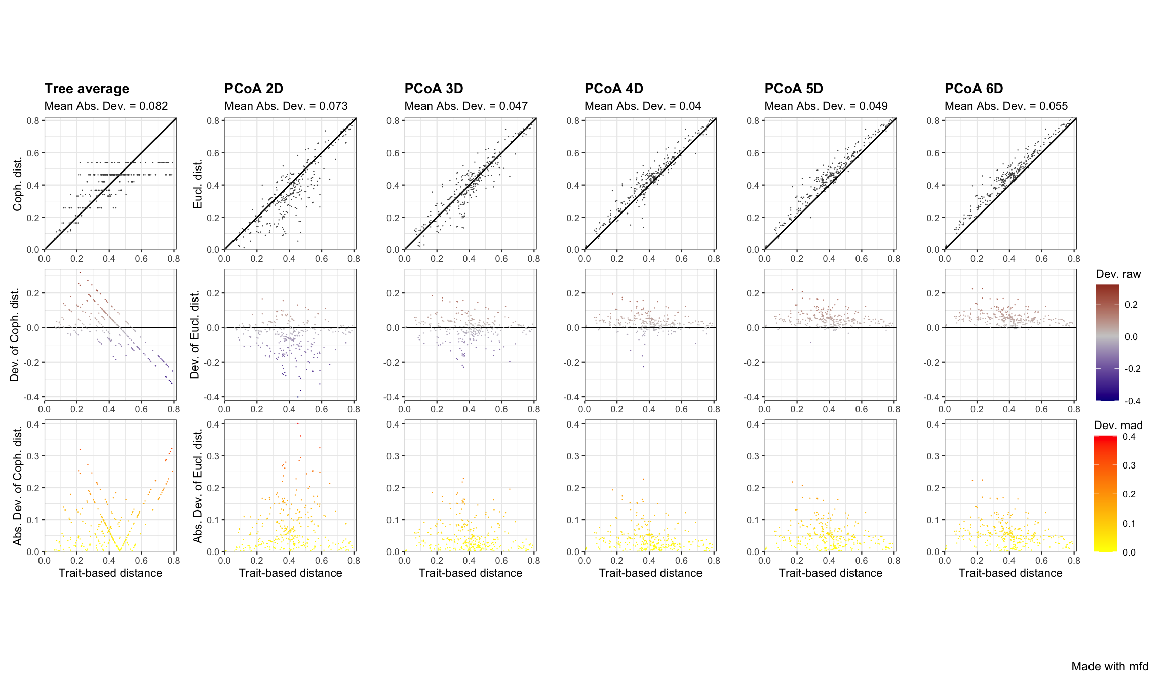
For the 2D space, on the top row there are a lot of points below the 1:1 lines, meaning that distances are overestimated in this multidimensional space. Looking at panels, we can see that the 4D space is the one in which points are the closest to the 1:1 line on the top row,and the closest to the x-axis for the two bottom rows, which reflects a better quality compared to other functional spaces / dendrogram. For the dendrogram, we can see on the top row that species pairs arrange in horizontal lines, meaning that different trait-based distances have then the same cophenetic distance on the dendrogram.

1.3.3. Testing the correlation between functional axes and traits

mFD allows to test for correlations between traits and functional axes and then illustrate possible correlations (continuous traits = linear model is computed and r² and associated p-value are returned; non-continuous traits = Kruskal-Wallis test is computed and eta2 statistic is returned). The function mFD::traits.faxes.cor() allows to test and plot correlation and needs the following arguments:

sp_tr is the species x traits data.frame
sp_faxes_coord is a matrix of species coordinates taken from the outputs of the mFD::quality.fspaces() function with columns representing axes on which functional space must be computed. For instance, in this tutorial, we will plot the functional space for 4 and 10 dimensions (cf. the two examples below). The whole sp_faxes_coord can be retrieved through the output of the mFD::quality.fspaces() function:

Code

sp_faxes_coord_fruits <- fspaces_quality_fruits$"details_fspaces"$"sp_pc_coord"

plot is a logical value indicating whether correlations should be illustrated or not. If this option is set to TRUE, traits-axis relationships are plotted through scatterplot for continuous traits and boxplot for non-continuous traits.

The function mFD::traits.faxes.cor() works as follows:

Code

fruits_tr_faxes <- mFD::traits.faxes.cor(
  sp_tr          = fruits_traits, 
  sp_faxes_coord = sp_faxes_coord_fruits[ , c("PC1", "PC2", "PC3", "PC4")], 
  plot           = TRUE)

We can print only traits with significant effect on position along one of the axis and look at the plots:

Code

## Print traits with significant effect ----
fruits_tr_faxes$"tr_faxes_stat"[which(fruits_tr_faxes$"tr_faxes_stat"$"p.value" < 0.05), ]

     trait axis           test stat value p.value
1     Size  PC1 Kruskal-Wallis eta2 0.308  0.0377
3     Size  PC3 Kruskal-Wallis eta2 0.326  0.0325
5    Plant  PC1 Kruskal-Wallis eta2 0.471  0.0049
6    Plant  PC2 Kruskal-Wallis eta2 0.382  0.0116
8    Plant  PC4 Kruskal-Wallis eta2 0.264  0.0360
9  Climate  PC1 Kruskal-Wallis eta2 0.731  0.0001
13    Seed  PC1 Kruskal-Wallis eta2 0.201  0.0402
14    Seed  PC2 Kruskal-Wallis eta2 0.593  0.0005
20   Sugar  PC4   Linear Model   r2 0.682  0.0000

## Plot ----
fruits_tr_faxes$"tr_faxes_plot"

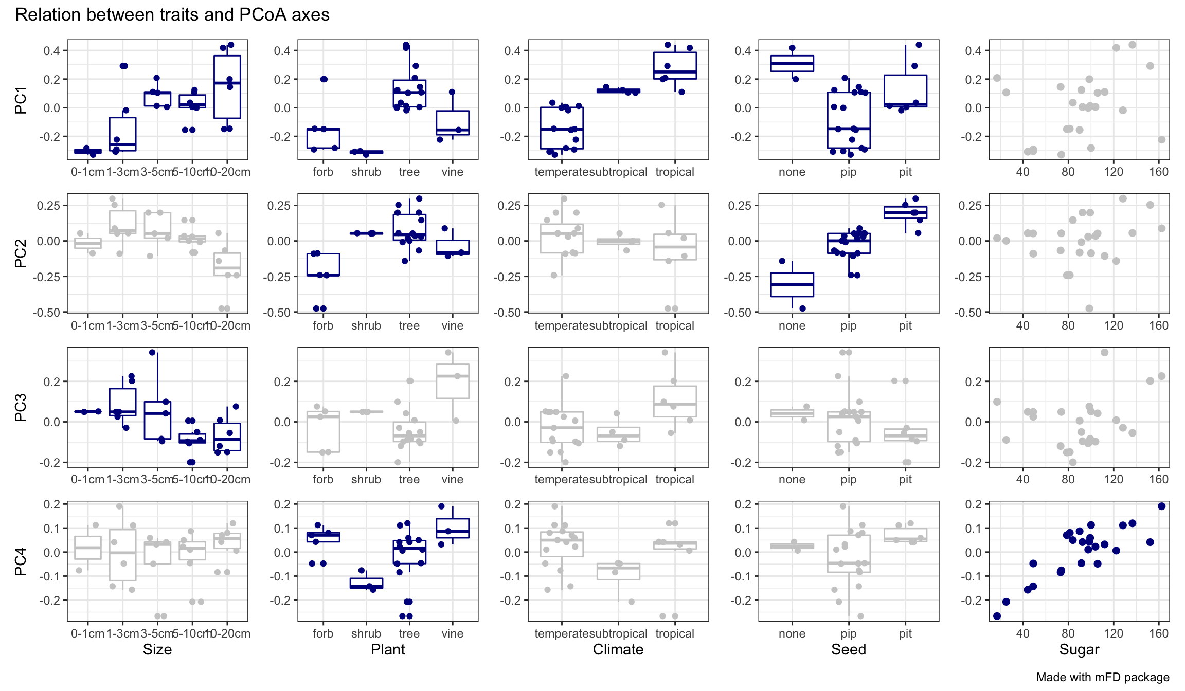
We can thus see that PC1 is mostly driven by Climate (temperate on the left and tropical on the right) and Plant Type (forb & shrub on the left vs tree & vine on the right) and Size (large fruits on the right) with weaker influence of Seed (eta2 < 0.25). Then, PC2 is mostly driven by Seed (no seed on the left and pit seed on the right) with weaker influence of Plant Type. PC3 is driven by only one trait, Size. And finally PC4 is mostly driven by Sugar (high sugar content on the right and low sugar content on the left) with a weaker influence of Plant Type.

1.4. Plotting the selected functional space and position of species

Once the user has selected the dimensionality of the functional space, mFD allows you to plot the given multidimensional functional space and the position of species in all 2-dimensions spaces made by pairs of axes.

The mFD::funct.space.plot() function allows to illustrate the position of all species along pairs of space axes.

This function allows to plot with many possibilities to change colors/shapes of each plotted element. Here are listed the main arguments:

sp_faxes_coord is a matrix of species coordinates taken from the outputs of the mFD::quality.fspaces() function with columns representing axes on which functional space must be computed. For instance, in this tutorial, we will plot the functional space for 4 and 10 dimensions (cf. the two examples below). The whole sp_faxes_coord can be retrieved through the output of the mFD::quality.fspaces() function:

Code

sp_faxes_coord_fruits <- fspaces_quality_fruits$"details_fspaces"$"sp_pc_coord"

faxes is a vector containing names of axes to plot. If set to NULL, the first four functional axes will be plotted.
faxes_nm is a vector containing labels of faxes (following faxes vector rank). If NULL, labels follow faxes vector names.
range_faxes is a vector to complete if the user wants to set specific limits for functional axes. If range_faxes = c(NA, NA), the range is computed according to the range of values among all axes.
plot_ch is a logical value used to draw or not the 2D convex-hull filled by the global pool of species. Color, fill and opacity of the convex hull can be chosen through other inputs, please refer to the function’s help.
plot_sp_nm is a vector containing species names to plot. If NULL, no species names plotted. Name size, color and font can be chosen through other inputs, please refer to the function’s help.
plot_vertices is a logical value used to plot or not vertices with a different shape than other species. Be careful these representations are 2D representations, thus vertices of the convex-hull in the n-multidimensional space can be close to the center of the hull projected in 2D. Color, fill, shape and size of vertices can be chosen through other inputs, please refer to the function’s help.
check_input is a recurrent argument in the mFD package. It defines whether inputs should be checked before computation or not. Possible error messages will thus be more understandable for the user than R error messages (Recommendation: set it as TRUE).
other inputs are used to chose color, fill, size, and shape of species from the global pool, please refer to the function’s help.

Here are the plots for the fruits & baskets dataset for the first four PCoA axis:

Code

big_plot <- mFD::funct.space.plot(
  sp_faxes_coord  = sp_faxes_coord_fruits[ , c("PC1", "PC2", "PC3", "PC4")],
  faxes           = c("PC1", "PC2", "PC3", "PC4"),
  name_file       = NULL,
  faxes_nm        = NULL,
  range_faxes     = c(NA, NA),
  plot_ch         = TRUE,
  plot_vertices   = TRUE,
  plot_sp_nm      = NULL,
  check_input     = TRUE)

big_plot$"patchwork"

Here, the convex-hull of the species pool is plotted in white and axis have the same range to get rid of bias based on different axis scales. Species being vertices of the 4D convex hull are in purple.

Part 2. Computing and plotting FD indices using the `mFD` package

The mFD::alpha.fd.multidim() function allows computing alpha and beta FD indices.

2.1. Computing and plotting alpha FD indices

Using the alpha.fd.multidim() function, you can compute up to nine alpha FD indices:

FDis Functional Dispersion: the biomass weighted deviation of species traits values from the center of the functional space filled by the assemblage i.e. the biomass-weighted mean distance to the biomass-weighted mean trait values of the assemblage.
FRic Functional Richness: the proportion of functional space filled by species of the studied assemblage, i.e. the volume inside the convex-hull shaping species. To compute FRic the number of species must be at least higher than the number of functional axis + 1.
FDiv Functional Divergence: the proportion of the biomass supported by the species with the most extreme functional traits i.e. the ones located close to the edge of the convex-hull filled by the assemblage.
FEve Functional Evenness: the regularity of biomass distribution in the functional space using the Minimum Spanning Tree linking all species present in the assemblage.
FSpe Functional Specialization: the biomass weighted mean distance to the mean position of species from the global pool (present in all assemblages).
FMPD Functional Mean Pairwise Distance: the mean weighted distance between all species pairs.
FNND Functional Mean Nearest Neighbour Distance: the weighted distance to the nearest neighbor within the assemblage.
FIde Functional Identity: the mean traits values for the assemblage. FIde is always computed when FDis is computed.
FOri Functional Originality: the weighted mean distance to the nearest species from the global species pool.

A cheat sheet on alpha FD indices is available here

In this Practice we will only compute five of them. The function is used as follow:

Code

alpha_fd_indices_fruits <- mFD::alpha.fd.multidim(
  sp_faxes_coord   = sp_faxes_coord_fruits[ , c("PC1", "PC2", "PC3", "PC4")],
  asb_sp_w         = baskets_fruits_weights,
  ind_vect         = c("fdis", "fric", "fdiv", 
                       "fspe", "fide"),
  scaling          = TRUE,
  check_input      = TRUE,
  details_returned = TRUE)

The arguments and their use are listed below:

sp_faxes_coord is the species coordinates matrix. This dataframe gathers only axis of the functional space you have chosen based on step 4.
asb_sp_w is the matrix linking species and assemblages they belong to (summarized in step 1).
ind_vect is a vector with names of diversity functional indices to compute.
scaling is a logical value indicating whether indices should be scaled between 0 and 1. If scaling is to be done, this argument must be set to TRUE.
check_input is a recurrent argument in the mFD package. It defines whether inputs should be checked before computation or not. Possible error messages will thus be more understandable for the user than R error messages (Recommendation: set it as TRUE).
details_returned is used if the user wants to store information that are used in graphical functions. If the user wants to plot FD indices, then details_returned must be set to TRUE.

N.B. Use lowercase letters to enter FD indices names

The function has two main outputs:

a data.frame gathering indices values in each assemblage (for FIde values, there are as many columns as there are axes to the studied functional space).

Code

fd_ind_values_fruits <- alpha_fd_indices_fruits$"functional_diversity_indices"
fd_ind_values_fruits

          sp_richn      fdis        fric      fdiv      fspe
basket_1         8 0.4763773 0.162830681 0.5514453 0.4127138
basket_2         8 0.7207823 0.162830681 0.8064809 0.5781232
basket_3         8 0.7416008 0.162830681 0.8089535 0.5888104
basket_4         8 0.2958614 0.007880372 0.6080409 0.3106937
basket_5         8 0.3673992 0.007880372 0.7288912 0.3488358
basket_6         8 0.8001980 0.147936148 0.8937934 0.7930809
basket_7         8 0.8121314 0.147936148 0.8989094 0.7443406
basket_8         8 0.4678159 0.036480112 0.7113688 0.6363814
basket_9         8 0.5577452 0.036480112 0.7787237 0.6309078
basket_10        8 0.5505783 0.025774304 0.7741681 0.4587432
             fide_PC1     fide_PC2    fide_PC3     fide_PC4
basket_1  -0.01473662 -0.009461738 -0.05670043 -0.001823969
basket_2   0.01887361 -0.061601373 -0.04427402  0.021249327
basket_3   0.04724418 -0.056571400 -0.03631846  0.018045257
basket_4   0.03994897  0.052581211 -0.08413271 -0.001343112
basket_5   0.02349573  0.039069220 -0.08187248 -0.010262902
basket_6   0.24320913 -0.114434642  0.01394977  0.025500282
basket_7   0.13341179 -0.183609095 -0.01782549  0.021494300
basket_8  -0.24497368  0.036194656  0.04748935 -0.038827673
basket_9  -0.21021559  0.029339706  0.05516746 -0.041392184
basket_10 -0.05375867 -0.005743348 -0.05649324  0.041191011

a details list of data.frames and lists gathering information such as coordinates of centroids, distances and identity of the nearest neighbour, distances to the centroid, etc. The user does not have to directly use it but it will be useful if FD indices are then plotted. It can be retrieved through:

Code

details_list_fruits <- alpha_fd_indices_fruits$"details"

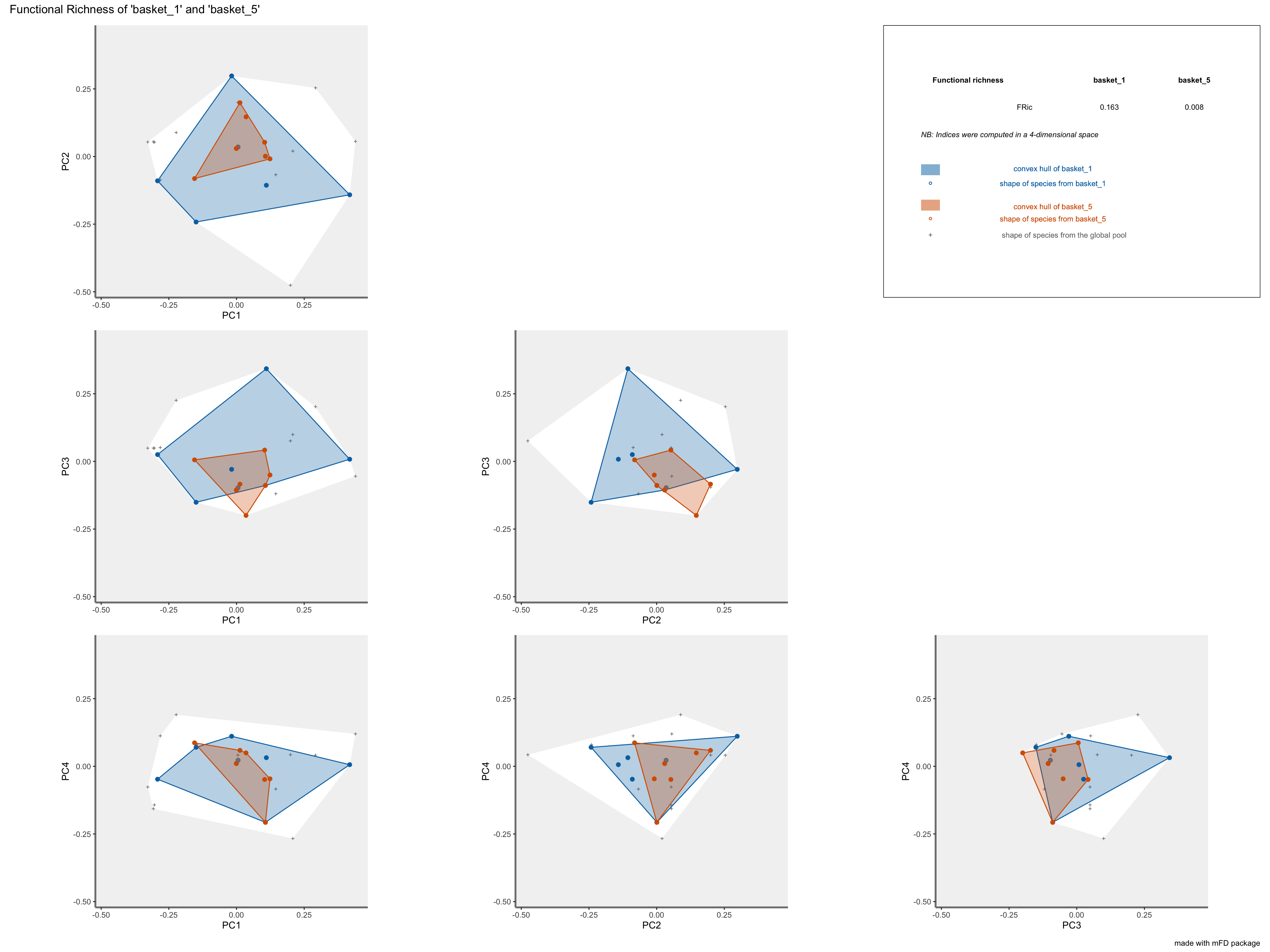
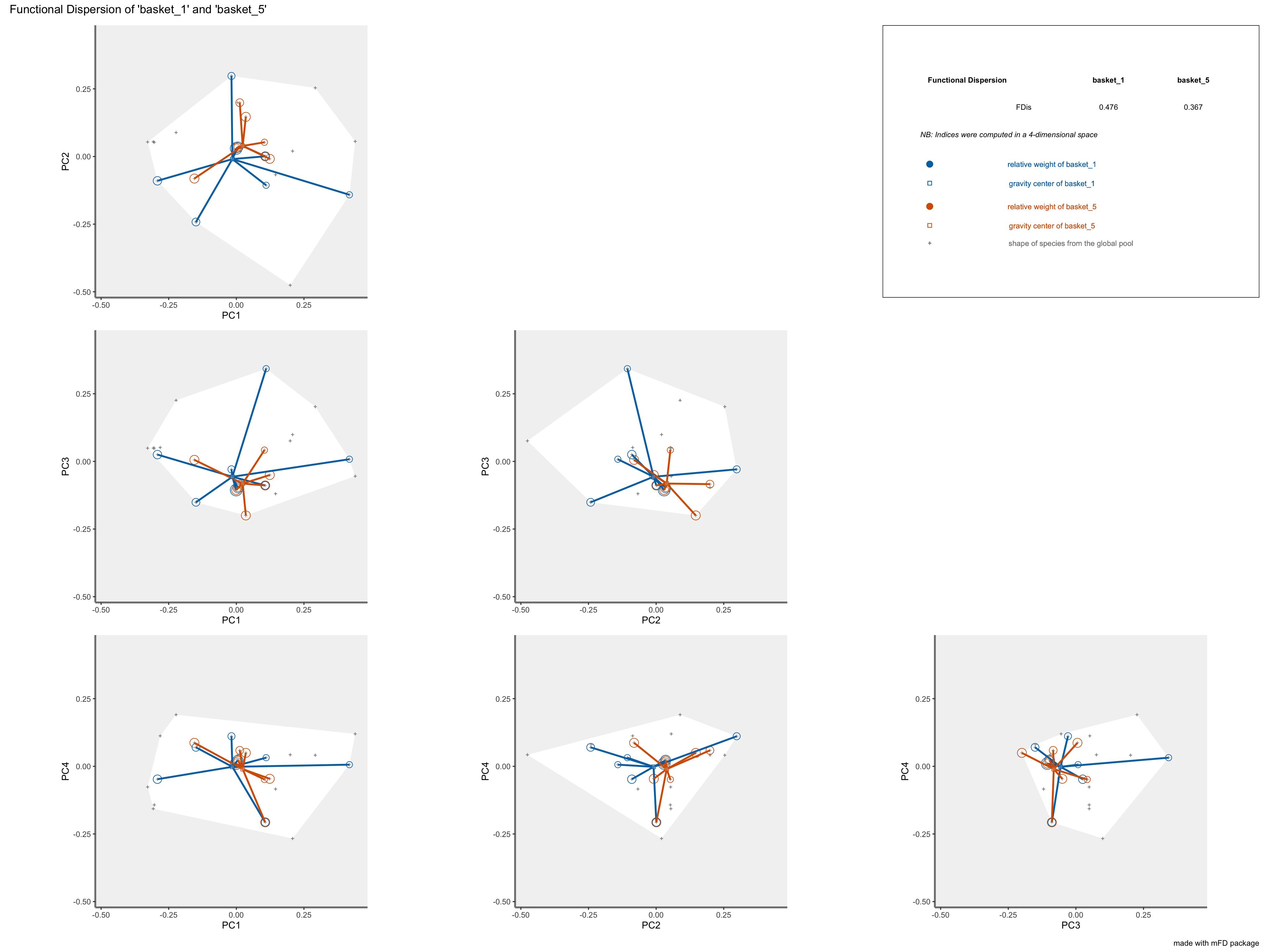
Then, you can plot functional indices using the mFD::alpha.multidim.plot() for up to two assemblages:

Code

plots_alpha <- mFD::alpha.multidim.plot(
  output_alpha_fd_multidim = alpha_fd_indices_fruits,
  plot_asb_nm              = c("basket_1", "basket_5"),
  ind_nm                   = c("fdis", "fric", "fdiv", 
                              "fspe", "fide"),
  faxes                    = NULL,
  faxes_nm                 = NULL,
  range_faxes              = c(NA, NA),
  plot_sp_nm               = NULL,
  save_file                = FALSE,
  check_input              = TRUE)

This function has a lot of arguments: most of them are graphical arguments allowing the user to chose colors, shapes, sizes, scales, etc. This tutorial only presents main arguments. To learn about the use of graphical arguments, check the function help file. The main arguments of this function are listed below:

output_alpha_fd_multidim is the output of the `mFD::alpha.fd.multidim() function.
plot_asb_nm is a vector gathering name(s) of assemblage(s) to plot.
ind_vect is a vector gathering FD indices to plot. Plots are available for FDis, FIde, FEve, FRic, FDiv, FOri, FSpe, and FNND.
faxes is a vector containing names of axes to plot. You can only plot from two to four axes labels for graphical reasons.
faxes_nm is a vector with axes labels if the user ants different axes labels than faxes ones.
range_faxes is a vector with minimum and maximum values for axes. If range_faxes = c(NA, NA), the range is computed according to the range of values among all axes, all axes having thus the same range. To have a fair representation of species positions in all plots, all axes must have the same range.
plot_sp_nm is a vector containing species names to plot. If NULL, then no name is plotted.
check_input is a recurrent argument in mFD. It defines whether inputs should be checked before computation or not. Possible error messages will thus be more understandable for the user than R error messages (Recommendation: set it as TRUE.
size, color, fill, and shape arguments for each component of the graphs i.e. species of the global pool, species of the studied assemblage(s), vertices, centroids and segments. If you have to plot two assemblages, then inputs should be formatted as follow: c(pool = ..., asb1 = ..., asb2 = ...) for inputs used for global pool and studied assemblages and c(asb1 = ..., asb2 = ...) for inputs used for studied assemblages only.

Then, using these arguments, here are the output plots for the fruits & baskets dataset:

FRic representation: the colored shapes reflect the convex-hull of the studied assemblages and the white shape reflects the convex-hull of the global pool of species:

Code

plots_alpha$"fric"$"patchwork"

FDiv representation: the gravity centers of vertices (i.e. species with the most extreme functional traits) of each assemblages are plotted as a square and a triangle. The two colored circles represent the mean distance of species to the gravity center for each assemblage. Species of each assemblage have different size given their relative weight into the assemblage.

Code

plots_alpha$"fdiv"$"patchwork"

FSpe representation: colored traits represent distances of each species from a given assemblage to the center of gravity of the global pool (i.e center of the functional space). the center of gravity is plotted with a purple diamond. Species of each assemblage have different size given their relative weight into the assemblage.

Code

plots_alpha$"fspe"$"patchwork"

FDis representation: colored traits represent distances of each species from a given assemblage to the center of gravity of species of the assemblage (defined by FIde values). The center of gravity of each assemblage is plotted using a square and a triangle. Species of each assemblage havedifferent size given their relative weight into the assemblage.

Code

plots_alpha$"fdis"$"patchwork"

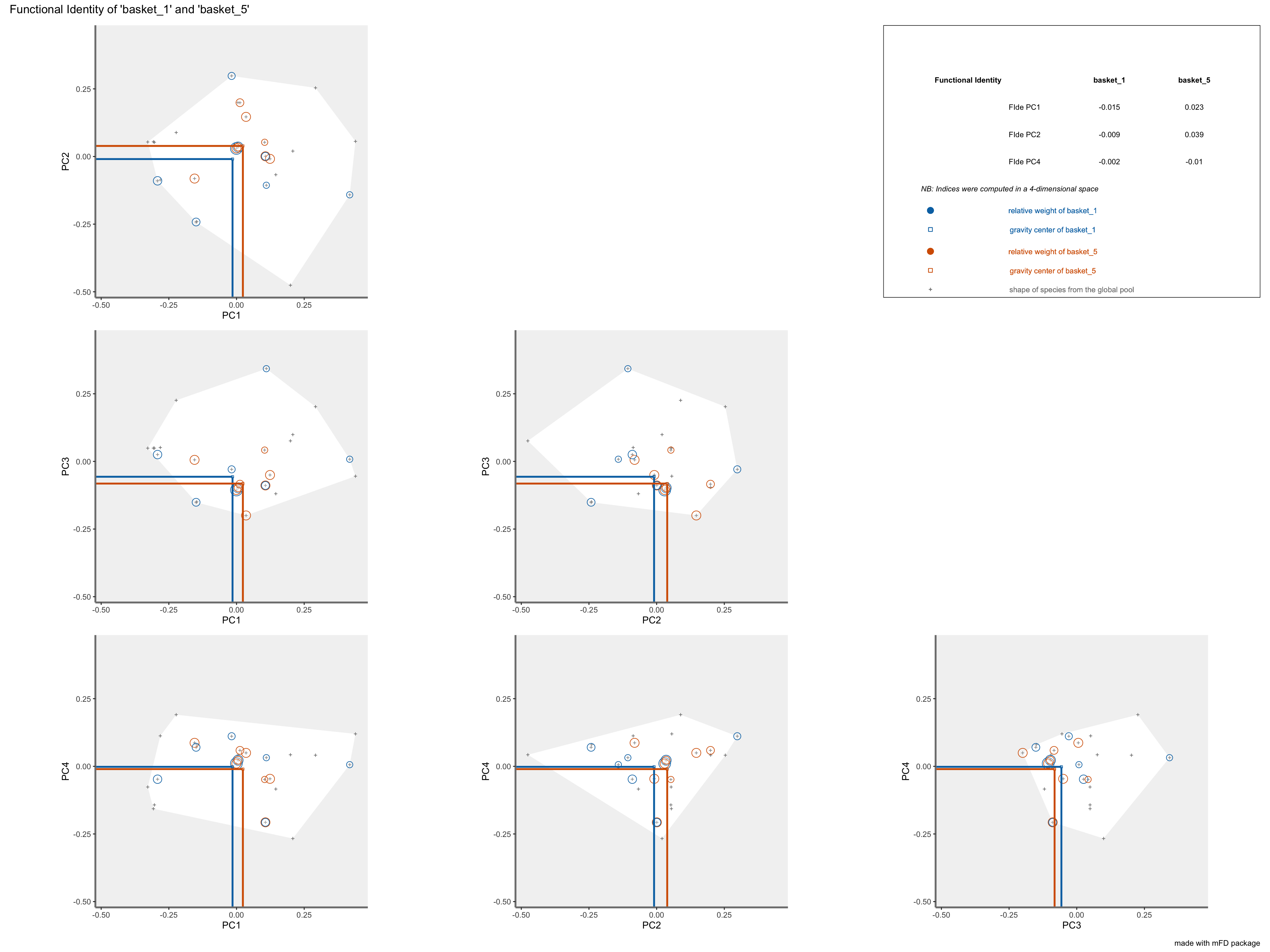
FIde representation:colored lines refer to the weighted average position of species of each assemblage along each axis. Species of each assemblage have different size given their relative weight into the assemblage.

Code

plots_alpha$"fide"$"patchwork"

N.B. Using the mFD package, you can plot more than two assemblages but not with the alpha.multidim.plot() function. There are several specific functions for each step of the plot: build the background of the plot (background.plot()), plot the pool of species you are working on (pool.plot()), plot species from the studied assemblages (species.plot()) function and lastly plot the wanted metric using related function (fric.plot(), fdiv.plot(), fide.plot(),fdis.plot(), feve.plot(), fnnd.plot(), fori.plot(), fspe.plot()). Plots for different axes combination can be gathered into a single plot using the panels.to.patchwork() function.

2.2. Computing and plotting beta FD indices

N.B. Some Mac OS X 10.15 may encounter some issues with the beta_*() functions.

mFD package allows you to compute beta diversity indices for each assemblage pairs following Villeger et al. 2013. For that we will use the mFD::beta.fd.multidim() function. This function can compute two families of functional beta diversity indices, either Jaccard or Sorensen.

In this example, we will use Jaccard index. For each assemblages pair, the dissimilarity index is decomposed into two additive components: turnover and nestedness-resultant.

NB The turnover component is the highest if there is no shared traits combination between the two assemblages. The nestedness component is the highest if one assemblage hosts a small subset of the functional strategies present in the other.

The mFD::beta.fd.multidim() function has the main following arguments:

Code

beta_fd_indices_fruits <- mFD::beta.fd.multidim(
      sp_faxes_coord   = sp_faxes_coord_fruits[ , c("PC1", "PC2", "PC3", "PC4")],
      asb_sp_occ       = asb_sp_fruits_occ,
      check_input      = TRUE,
      beta_family      = c("Jaccard"),
      details_returned = TRUE)

sp_faxes_coord is the species coordinates matrix. This dataframe gathers only axis of the functional space you have chosen based on step 4.
asb_sp_occ is the matrix of occurrence (coded as 0/1) of species assemblages (summarized in step 1).
check_input is a recurrent argument in the mFD package. It defines whether inputs should be checked before computation or not. Possible error messages will thus be more understandable for the user than R error messages (Recommendation: set it as TRUE.
beta_family a character string for the type of beta-diversity index to compute, it can either be Jaccard or Sorensen.
details_returned is a logical value indicating whether details of outputs must be stored. It should be stored if you plan to use the graphical function to illustrate beta diversity indices thereafter.
There are also other arguments for parallelisation options. Check the function help file for more explanation.

The function returns a list containing:

a dist object with beta indices values for each pair of assemblages:

Code

head(beta_fd_indices_fruits$"pairasb_fbd_indices", 10)

$jac_diss
              basket_1     basket_2     basket_3     basket_4
basket_2  3.920303e-15                                       
basket_3  3.920303e-15 3.920303e-15                          
basket_4  9.654002e-01 9.654002e-01 9.654002e-01             
basket_5  9.654002e-01 9.654002e-01 9.654002e-01 0.000000e+00
basket_6  8.701848e-01 8.701848e-01 8.701848e-01 9.972695e-01
basket_7  8.701848e-01 8.701848e-01 8.701848e-01 9.972695e-01
basket_8  9.797030e-01 9.797030e-01 9.797030e-01 1.000000e+00
basket_9  9.797030e-01 9.797030e-01 9.797030e-01 1.000000e+00
basket_10 9.151338e-01 9.151338e-01 9.151338e-01 9.303584e-01
              basket_5     basket_6     basket_7     basket_8
basket_2                                                     
basket_3                                                     
basket_4                                                     
basket_5                                                     
basket_6  9.972695e-01                                       
basket_7  9.972695e-01 0.000000e+00                          
basket_8  1.000000e+00 1.000000e+00 1.000000e+00             
basket_9  1.000000e+00 1.000000e+00 1.000000e+00 0.000000e+00
basket_10 9.303584e-01 9.983508e-01 9.983508e-01 9.702788e-01
              basket_9
basket_2              
basket_3              
basket_4              
basket_5              
basket_6              
basket_7              
basket_8              
basket_9              
basket_10 9.702788e-01

$jac_turn
              basket_1     basket_2     basket_3     basket_4
basket_2  3.920303e-15                                       
basket_3  3.920303e-15 3.920303e-15                          
basket_4  4.320333e-01 4.320333e-01 4.320333e-01             
basket_5  4.320333e-01 4.320333e-01 4.320333e-01 0.000000e+00
basket_6  8.627528e-01 8.627528e-01 8.627528e-01 9.723344e-01
basket_7  8.627528e-01 8.627528e-01 8.627528e-01 9.723344e-01
basket_8  9.425331e-01 9.425331e-01 9.425331e-01 1.000000e+00
basket_9  9.425331e-01 9.425331e-01 9.425331e-01 1.000000e+00
basket_10 5.990146e-01 5.990146e-01 5.990146e-01 8.385233e-01
              basket_5     basket_6     basket_7     basket_8
basket_2                                                     
basket_3                                                     
basket_4                                                     
basket_5                                                     
basket_6  9.723344e-01                                       
basket_7  9.723344e-01 0.000000e+00                          
basket_8  1.000000e+00 1.000000e+00 1.000000e+00             
basket_9  1.000000e+00 1.000000e+00 1.000000e+00 0.000000e+00
basket_10 8.385233e-01 9.944208e-01 9.944208e-01 9.638833e-01
              basket_9
basket_2              
basket_3              
basket_4              
basket_5              
basket_6              
basket_7              
basket_8              
basket_9              
basket_10 9.638833e-01

$jac_nest
             basket_1    basket_2    basket_3    basket_4    basket_5
basket_2  0.000000000                                                
basket_3  0.000000000 0.000000000                                    
basket_4  0.533366944 0.533366944 0.533366944                        
basket_5  0.533366944 0.533366944 0.533366944 0.000000000            
basket_6  0.007431956 0.007431956 0.007431956 0.024935183 0.024935183
basket_7  0.007431956 0.007431956 0.007431956 0.024935183 0.024935183
basket_8  0.037169839 0.037169839 0.037169839 0.000000000 0.000000000
basket_9  0.037169839 0.037169839 0.037169839 0.000000000 0.000000000
basket_10 0.316119149 0.316119149 0.316119149 0.091835053 0.091835053
             basket_6    basket_7    basket_8    basket_9
basket_2                                                 
basket_3                                                 
basket_4                                                 
basket_5                                                 
basket_6                                                 
basket_7  0.000000000                                    
basket_8  0.000000000 0.000000000                        
basket_9  0.000000000 0.000000000 0.000000000            
basket_10 0.003930032 0.003930032 0.006395544 0.006395544

a list containing details such as inputs, vertices of the global pool and of each assemblage and FRic values for each assemblage

Code

beta_fd_indices_fruits$"details"

$inputs
$inputs$sp_faxes_coord
                        PC1           PC2          PC3          PC4
apple          0.0055715265  0.0350421604 -0.097471237  0.022402932
apricot        0.0051324906  0.1993950375 -0.095659935  0.041498534
banana         0.4180172546 -0.1414728845  0.008086992  0.006165812
currant       -0.3278449659  0.0536374098  0.049052945 -0.076408888
blackberry    -0.3034346496  0.0526909897  0.049135314 -0.142658171
blueberry     -0.2815708070 -0.0866665191  0.051316336  0.112502412
cherry        -0.0180809780  0.2978695529 -0.029313202  0.111166444
grape         -0.2228504050  0.0885963887  0.225751135  0.190718259
grapefruit     0.1450603259 -0.0673074635 -0.119455606 -0.084037260
kiwifruit     -0.1550698937 -0.0814958746  0.005740138  0.086787104
lemon          0.1067949113  0.0007714157 -0.088895714 -0.207026513
lime           0.2079695595  0.0199956576  0.099157708 -0.266782185
litchi         0.2917434196  0.2537533311  0.202206065  0.041136776
mango          0.4393412201  0.0559467870 -0.054626734  0.119804224
melon         -0.1493941692 -0.2420723462 -0.151024241  0.070247222
orange         0.1236282949 -0.0086604744 -0.050235439 -0.046156784
passion_fruit  0.1101264243 -0.1062790540  0.342728218  0.031929461
peach          0.0351203321  0.1465415655 -0.199699124  0.049647666
pear          -0.0005886084  0.0297927029 -0.105703762  0.010290065
pineapple      0.1991811945 -0.4756825960  0.075904777  0.042696533
plum           0.0126064681  0.1989177835 -0.084010036  0.058965350
raspberry     -0.3070933066  0.0543878274  0.049178225 -0.156730076
strawberry    -0.2917242495 -0.0898440618  0.025237344 -0.047647147
tangerine      0.1039035285  0.0526165085  0.041894666 -0.048619225
water_melon   -0.1465449176 -0.2404738440 -0.149294834  0.080107453

$inputs$asb_sp_occ
          apple apricot banana currant blackberry blueberry cherry
basket_1      1       0      1       0          0         0      1
basket_2      1       0      1       0          0         0      1
basket_3      1       0      1       0          0         0      1
basket_4      1       0      0       0          0         0      0
basket_5      1       0      0       0          0         0      0
basket_6      1       0      1       0          0         0      0
basket_7      1       0      1       0          0         0      0
basket_8      0       0      0       1          1         1      1
basket_9      0       0      0       1          1         1      1
basket_10     1       1      0       0          0         0      0
          grape grapefruit kiwifruit lemon lime litchi mango melon
basket_1      0          0         0     1    0      0     0     1
basket_2      0          0         0     1    0      0     0     1
basket_3      0          0         0     1    0      0     0     1
basket_4      0          0         1     1    0      0     0     0
basket_5      0          0         1     1    0      0     0     0
basket_6      0          0         0     0    1      1     1     0
basket_7      0          0         0     0    1      1     1     0
basket_8      1          0         0     1    0      0     0     0
basket_9      1          0         0     1    0      0     0     0
basket_10     1          1         0     0    0      0     0     1
          orange passion_fruit peach pear pineapple plum raspberry
basket_1       0             1     0    1         0    0         0
basket_2       0             1     0    1         0    0         0
basket_3       0             1     0    1         0    0         0
basket_4       1             0     1    1         0    1         0
basket_5       1             0     1    1         0    1         0
basket_6       1             0     0    0         1    0         0
basket_7       1             0     0    0         1    0         0
basket_8       0             0     0    0         0    0         1
basket_9       0             0     0    0         0    0         1
basket_10      0             0     0    1         0    1         0
          strawberry tangerine water_melon
basket_1           1         0           0
basket_2           1         0           0
basket_3           1         0           0
basket_4           0         1           0
basket_5           0         1           0
basket_6           0         0           1
basket_7           0         0           1
basket_8           1         0           0
basket_9           1         0           0
basket_10          1         0           0


$pool_vertices
 [1] "grape"         "lemon"         "water_melon"   "banana"       
 [5] "raspberry"     "cherry"        "blueberry"     "grapefruit"   
 [9] "melon"         "strawberry"    "peach"         "apricot"      
[13] "passion_fruit" "litchi"        "lime"          "pineapple"    
[17] "mango"         "currant"      

$asb_FRic
   basket_1    basket_2    basket_3    basket_4    basket_5 
0.162830681 0.162830681 0.162830681 0.007880372 0.007880372 
   basket_6    basket_7    basket_8    basket_9   basket_10 
0.147936148 0.147936148 0.036480112 0.036480112 0.025774304 

$asb_vertices
$asb_vertices$basket_1
[1] "lemon"         "melon"         "pear"          "apple"        
[5] "passion_fruit" "cherry"        "strawberry"    "banana"       

$asb_vertices$basket_2
[1] "lemon"         "melon"         "pear"          "apple"        
[5] "passion_fruit" "cherry"        "strawberry"    "banana"       

$asb_vertices$basket_3
[1] "lemon"         "melon"         "pear"          "apple"        
[5] "passion_fruit" "cherry"        "strawberry"    "banana"       

$asb_vertices$basket_4
[1] "peach"     "lemon"     "tangerine" "pear"      "plum"     
[6] "orange"    "kiwifruit"

$asb_vertices$basket_5
[1] "peach"     "lemon"     "tangerine" "pear"      "plum"     
[6] "orange"    "kiwifruit"

$asb_vertices$basket_6
[1] "litchi"      "lime"        "apple"       "banana"     
[5] "orange"      "pineapple"   "mango"       "water_melon"

$asb_vertices$basket_7
[1] "litchi"      "lime"        "apple"       "banana"     
[5] "orange"      "pineapple"   "mango"       "water_melon"

$asb_vertices$basket_8
[1] "strawberry" "blueberry"  "raspberry"  "cherry"     "grape"     
[6] "lemon"      "currant"   

$asb_vertices$basket_9
[1] "strawberry" "blueberry"  "raspberry"  "cherry"     "grape"     
[6] "lemon"      "currant"   

$asb_vertices$basket_10
[1] "grape"      "melon"      "plum"       "apricot"    "grapefruit"
[6] "strawberry"

a vector containing the FRic value for each assemblage retrieved through the details_beta list:

Code

beta_fd_indices_fruits$"details"$"asb_FRic"

   basket_1    basket_2    basket_3    basket_4    basket_5 
0.162830681 0.162830681 0.162830681 0.007880372 0.007880372 
   basket_6    basket_7    basket_8    basket_9   basket_10 
0.147936148 0.147936148 0.036480112 0.036480112 0.025774304

a list of vectors containing names of species being vertices of the convex hull for each assemblage retrieved through the details_beta list:

beta_fd_indices_fruits$"details"$"asb_vertices"

$basket_1
[1] "lemon"         "melon"         "pear"          "apple"        
[5] "passion_fruit" "cherry"        "strawberry"    "banana"       

$basket_2
[1] "lemon"         "melon"         "pear"          "apple"        
[5] "passion_fruit" "cherry"        "strawberry"    "banana"       

$basket_3
[1] "lemon"         "melon"         "pear"          "apple"        
[5] "passion_fruit" "cherry"        "strawberry"    "banana"       

$basket_4
[1] "peach"     "lemon"     "tangerine" "pear"      "plum"     
[6] "orange"    "kiwifruit"

$basket_5
[1] "peach"     "lemon"     "tangerine" "pear"      "plum"     
[6] "orange"    "kiwifruit"

$basket_6
[1] "litchi"      "lime"        "apple"       "banana"     
[5] "orange"      "pineapple"   "mango"       "water_melon"

$basket_7
[1] "litchi"      "lime"        "apple"       "banana"     
[5] "orange"      "pineapple"   "mango"       "water_melon"

$basket_8
[1] "strawberry" "blueberry"  "raspberry"  "cherry"     "grape"     
[6] "lemon"      "currant"   

$basket_9
[1] "strawberry" "blueberry"  "raspberry"  "cherry"     "grape"     
[6] "lemon"      "currant"   

$basket_10
[1] "grape"      "melon"      "plum"       "apricot"    "grapefruit"
[6] "strawberry"

Then, the package allows the user to illustrate functional beta-diversity indices for a pair of assemblages in a multidimensional space using the mFD::beta.multidim.plot() function. The output of this function is a figure showing the overlap between convex hulls shaping each of the two species assemblages.

The plotting function has a large number of arguments, allowing the user to chose graphical options. Only main arguments are listed below:

Code

beta_plot_fruits <- mFD::beta.multidim.plot(
  output_beta_fd_multidim = beta_fd_indices_fruits,
  plot_asb_nm             = c("basket_1", "basket_4"),
  beta_family             = c("Jaccard"),
  plot_sp_nm              = c("apple", "lemon", "pear"),
  faxes                   = paste0("PC", 1:4),
  name_file               = NULL,
  faxes_nm                = NULL,
  range_faxes             = c(NA, NA),
  check_input             = TRUE)

output_beta_fd_multidim is the output of the mFD::beta.fd.multidim() function retrieved before as beta_fd_indices.
plot_asb_nm is a vector containing the name of the two assemblages to plot. Here plots of indices will be shown for basket_1 and basket_4.
beta_family refers to the family of the plotted index. It must be the same as the family chosen to compute beta functional indices values with the mFD::beta.fd.multidim() function.
plot_sp_nm is a vector containing the names of species the user want to plot, if any. If no the user does not want to plot any species name, then this argument must be set up to NULL. Here, apple, cherry and lemon will be plotted on the graph.
faxes is a vector containing the names of the functional axes of the plotted functional space. Here, the figure will be plotted for PC1, PC2 and PC3. This function allows you to plot between two and four axes for graphical reasons.
name_file is a character string with the name of the file to save the figure (without extension). If the user does not want to save the file and only display it, this argument must be set up to NULL.
faxes_nm is a vector containing the axes labels for the figure if the user wants to set up different labels than those contained in faxes.
range_faxes is a vector with minimum and maximum values of functional axes. To have a fair representation of the position of species in all plots, axes should have the same range. If the user wants the range to be computed according to the range of values among all axes, this argument must be set up to c(NA, NA).
check_input is a recurrent argument in the mFD package. It defines whether inputs should be checked before computation or not. Possible error messages will thus be more understandable for the user than R error messages (Recommendation: set it as TRUE)
Others arguments to set up colors, shapes, sizes and, text fonts are also available. For more information about them, read the function help file.

Then, the function returns each graph for each functional axes combination and also a multipanel plot with all combinations of axes and the graph caption. Here is the multipanel for the fruits exaample:

beta_plot_fruits$"patchwork"

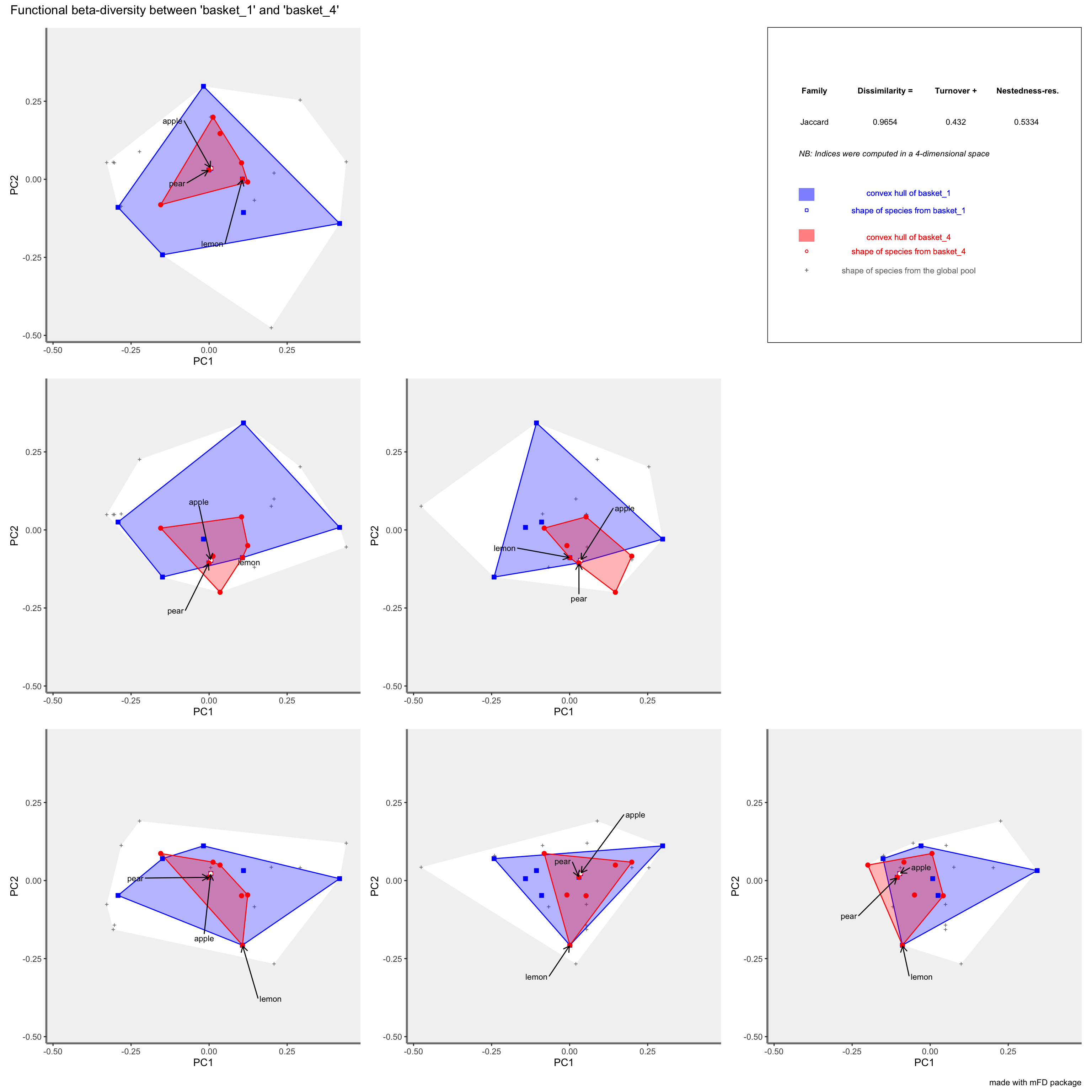
For each assemblage, the associated convex hull is plotted in a different colour and indices values are printed on the right corner of the plot. Vertices of the convex hull of a given assemblage can be plotted with a different symbol such as in this example. Species of all assemblages are plotted with gray cross and the associated convex hull is plotted in white.

Part 3. Functional rarity

In this part we’ll be using our built functional space to compute functional originality indices. The questions we’ll answer are:

What are functionally distinct fruits compared to all fruits together?
Are some of these fruits distinct at regional scale but not when looking at specific baskets?

3.1 Components of functional rarity: trait originality and rarity

Functional originality indices (also named functional rarity indices) measures how different are the trait of a target species compared to other ones among a set. Their idea is analogous to the rarity concept in terms of abundance: some species are rare because they show low abundance, some are common because of their high abundance. Well, functionally original species are original because they display trait values distant from most other species.

The indices were initially proposed as complimentary facets: one for “classical” rarity and one for trait “rarity” (= originality) Violle et al. 2017. With this framework, a species could be either rare or common, with either original or common traits. All combinations are possible. For example a species can be rare in abundance but have common traits. A species could also be common in abundance but original in terms of traits.

Violle et al. (2014) further declined the framework along two spatial scales, local and regional. The local scale is scale of the site or the assemblage, where species interact directly. The regional scale is the species pools scale, containing all species occurring in a given set of assemblages.

This initial framework thus contained 16 different possibilities between the different kinds of rarity (trait or abundance) and the spatial scales.

3.2 Different indices of functional rarity

One specificity of functional rarity indices is that we compute them on a species basis and not per sites. This means that for each species we will get one value.

3.2.1 Functional originality indices

The two proposed indices of functional originality are functional distinctiveness (Di) and functional uniqueness (Ui). They were initially envisioned at different spatial scales, with functional distinctiveness computed at local scale (and considering abundance) while functional uniqueness was to be computed at regional scales (without considering abundances).

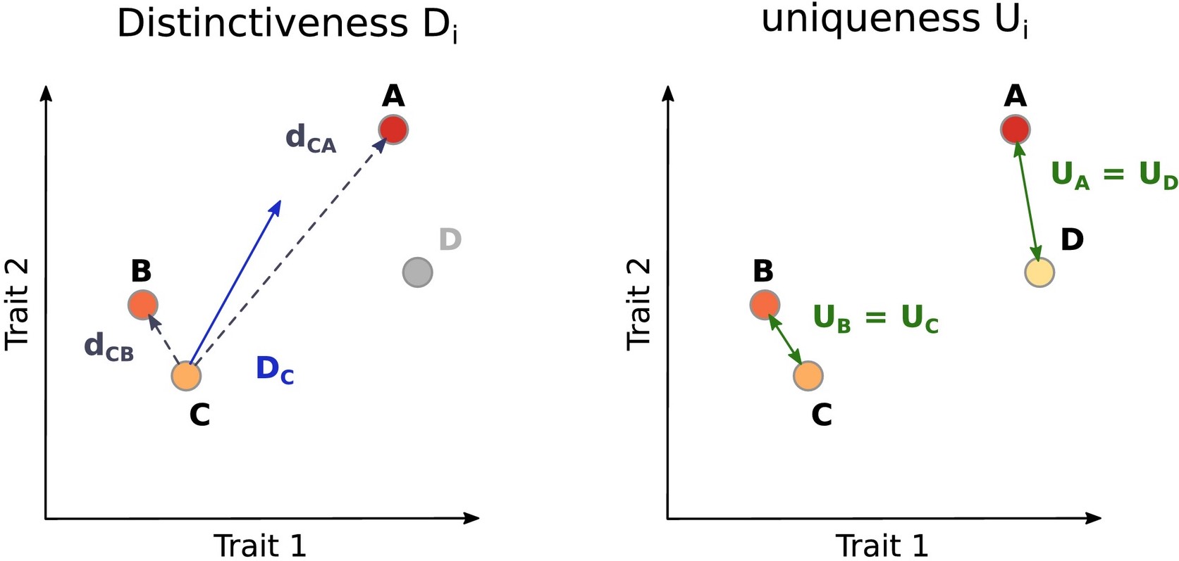
Scheme showing how Distinctiveness (Di) and Uniqueness (Ui) are computed

Functional distinctiveness is the mean of dissimilarity of the focal species to all the other species of the set of interest. It can be abundance-weighted if needed.

Functional uniqueness is the smallest dissimilarity that exists between the focal species and the all other species in the set. It does not consider the abundance of any species.

3.2.1 Rarity indices indices

The two proposed indices of rarity are scarcity (Si) and restrictedness. They are envisioned at different spatial scales because scarcity is directly computed from local species relative abundance while restrictedness is computed at regional scales considering all sites a species can occupy.

Scarcity is proportional to the relative abundance of the species. It gets close to one when the species is (relatively) rare and close to 0 when its dominant.

Restrictedness is 1 minus the ratio of sites a species occupy over the total number of sites.

3.3 Computing functional rarity

To compute functional rarity indices we will use two object: a functional dissimilarity matrix and a site-species matrix. We will be reusing the ones we defined in part 1 for that.

Because the funrar package follows strictly the framework defined by Violle et al. (2017), we have to consider the spatial scale at which we compute distinctiveness and uniqueness.

3.3.1 Functional originality at regional scale

At regional scale, we can compute distinctiveness using the distinctiveness_global() function. The first argument should be a functional dissimilarity matrix and the second argument gives the name of the output column.

library("funrar")

sp_di <- distinctiveness_global(sp_dist_fruits, di_name = "distinctiveness")

head(sp_di)

     species distinctiveness
1      apple       0.2930460
2    apricot       0.3421360
3     banana       0.4972814
4    currant       0.4496738
5 blackberry       0.4272436
6  blueberry       0.4264538

dim(sp_di)

[1] 25  2

We get one value of distinctiveness per species. It only considers the functional dissimilarity of all species in the dissimilarity matrix without considering their spatial distributions. We get one value of distinctiveness per species.

summary(sp_di)

quantile(sp_di$distinctiveness, probs = seq(0, 1, by = 0.1))

subset(sp_di, distinctiveness >= 0.48)

When looking at the most distinct fruits we see that banana, litchi, and pineapple, are the most distinct from their characteristics.

For the choice or dissimilarity matrix we can use the raw dissimilarity matrix computed directly on raw traits values among species, as we did here. Another option would be to compute a new functional dissimilarity matrix based on the selected functional axes. One advantage of the latter is that it already takes into account the correlation between traits.

Let’s recompute regional functional distinctiveness based on the four selected functional axes. Because the space comes from a PCA, we can directly use euclidean distance.

new_dissim <- dist(sp_faxes_coord_fruits[, c("PC1", "PC2", "PC3", "PC4")])

sp_di_alt <- distinctiveness_global(new_dissim, di_name = "alt_di")

We can now compare both distinctiveness values.

sp_all_di <- merge(sp_di, sp_di_alt, by = "species")

plot(sp_all_di$distinctiveness, sp_all_di$alt_di)

cor.test(sp_all_di$distinctiveness, sp_all_di$alt_di)


    Pearson's product-moment correlation

data:  sp_all_di$distinctiveness and sp_all_di$alt_di
t = 17.91, df = 23, p-value = 5.281e-15
alternative hypothesis: true correlation is not equal to 0
95 percent confidence interval:
 0.9232161 0.9851024
sample estimates:
      cor 
0.9659697

Both seems very correlated, so in our case using either one should be fine. However, it can be better to use dissimilarity based on a reduced number of well-defined axes because: (1) there are more interpretable thanks to the multivariate analysis, (2) the first one contain de most information, (3) they explicitly take into account potentially strong correlations between provided traits. We’ll stick here with raw dissimilarity for the sake of simplicity.

To compute uniqueness at regional scale we also need the regional level functional dissimilarity matrix with the uniqueness() function, and the site-species matrix:

sp_ui <- uniqueness(
  pres_matrix = baskets_fruits_weights,
  as.matrix(sp_dist_fruits)
)

head(sp_ui)
quantile(sp_ui$Ui, probs = seq(0, 1, by = 0.1))

subset(sp_ui, Ui >= 0.21)

Note that we have to transform the dissimilarity object sp_dist_fruits into a matrix explicitly so that the function uniqueness() works.

Based on these results we see that banana, passion fruit, and pineapple are the most isolated fruits in the functional space. Meaning that they have the most distant nearest neighbors.

So we see that some species can be regionally distinct and regionally unique (banana and pineapple), while some can be not so regionally distinct but regionally unique (passion fruit).

3.3.2 Functional originality at local scale

At local scale we can use similar logic but we will obtain one value per species per site.

For distinctiveness we can use the distinctiveness() function:

sp_local_di <- distinctiveness(
  baskets_fruits_weights, as.matrix(sp_dist_fruits)
)

sp_local_di[1:6, 1:6]

             apple apricot    banana currant blackberry blueberry
basket_1 0.1977721      NA 0.4642749      NA         NA        NA
basket_2 0.2852373      NA 0.5243089      NA         NA        NA
basket_3 0.2902663      NA 0.5219277      NA         NA        NA
basket_4 0.1136474      NA        NA      NA         NA        NA
basket_5 0.1393697      NA        NA      NA         NA        NA
basket_6 0.4138809      NA 0.3063492      NA         NA        NA

identical(dim(sp_local_di), dim(baskets_fruits_weights))

[1] TRUE

Note: because we provided a site-species matrix that contained “abundance” values (here the weights of the fruits in our baskets), the distinctiveness() is going to use them in its computation. If we want it not to consider abundances we need to convert the site-species matrix into a presence-absence matrix.

We get exactly the same number of sites and species as provided in the lists of baskets. Looking at the first column we see that the distinctiveness of apple varies a lot. Let’s see if can see how much it varies and why.

sp_local_di[, 1]

 basket_1  basket_2  basket_3  basket_4  basket_5  basket_6  basket_7 
0.1977721 0.2852373 0.2902663 0.1136474 0.1393697 0.4138809 0.3861698 
 basket_8  basket_9 basket_10 
       NA        NA 0.2313228

It varies from around 0.11 in basket 4 to up to 0.41 in basket 6. We can lookup the composition of these baskets to understand why:

baskets_fruits_weights[c(4, 6),]

         apple apricot banana currant blackberry blueberry cherry
basket_4   300       0      0       0          0         0      0
basket_6   100       0    200       0          0         0      0
         grape grapefruit kiwifruit lemon lime litchi mango melon
basket_4     0          0       100   100    0      0     0     0
basket_6     0          0         0     0  200    200   500     0
         orange passion_fruit peach pear pineapple plum raspberry
basket_4    400             0   300  400         0  200         0
basket_6    100             0     0    0       500    0         0
         strawberry tangerine water_melon
basket_4          0       200           0
basket_6          0         0         200

We can see that basket 4 contains fruits of similar size, origin and sweetness of apples: peach, pear, plums. This decreases the local distinctiveness of apples. While basket 6 contains more tropical fruits that are quite different in terms of size and sugar from apples.

To compute uniqueness at the site scale, we must use a more complex expression as it was not envisioned for local computation:

basket_ui <- apply(
  baskets_fruits_weights, 1,
  function(single_site, dist_m) {
    single_site = single_site[single_site > 0 & !is.na(single_site)]
    uniqueness(t(as.matrix(single_site)), dist_m)
  }, dist_m = as.matrix(sp_dist_fruits)
)

head(basket_ui[1])

$basket_1
        species          Ui
1         apple 0.008791209
2        banana 0.375274725
3        cherry 0.233379121
4         lemon 0.199587912
5         melon 0.190796703
6 passion_fruit 0.414148352
7          pear 0.008791209
8    strawberry 0.190796703

As we had to manually build the function to compute the local uniqueness the results are strangely formatted.

We provide here a function that can help them to be more easily read:

basket_ui <- lapply(names(basket_ui), function(x) {
  single_basket = basket_ui[[x]]
  single_basket$site = x
  
  return(single_basket)
})

basket_ui <- do.call(rbind, basket_ui)[, c(3, 1, 2)]

Then we can again look at the apple to see how its uniqueness varies across baskets.

subset(basket_ui, species == "apple")

        site species          Ui
1   basket_1   apple 0.008791209
9   basket_2   apple 0.008791209
17  basket_3   apple 0.008791209
25  basket_4   apple 0.008791209
33  basket_5   apple 0.008791209
41  basket_6   apple 0.117170330
49  basket_7   apple 0.117170330
73 basket_10   apple 0.008791209

We see that apple have the same uniqueness everywhere but in baskets 6 and 7. This means that it has the same nearest neighbor (in functional space) across all of these baskets. But that its closest neighbor is further away in baskets 6 and 7.

3.3.3 Rarity indices

Because rarity indices included in this framework are directly tied to specific spatial scales, we will compute them only at their respective spatial scales.

Similarly to functional originality indices, the functions to compute rarity indices follow their names. So we can use the scarcity() function to compute scarcity:

si = scarcity(baskets_fruits_weights)

Because scarcity needs relative abundances we get prompted by a message asking us to check if our data is relative. We will use make_relative() to transform the site-species matrix to a relative abundance matrix.

rel_weights = make_relative(baskets_fruits_weights)

si = scarcity(rel_weights)

si[1:4, 1:4]

             apple apricot    banana currant
basket_1 0.3298770      NA 0.7578583      NA
basket_2 0.5743492      NA 0.3298770      NA
basket_3 0.5743492      NA 0.2500000      NA
basket_4 0.4352753      NA        NA      NA

summary(si)

     apple           apricot           banana          currant      
 Min.   :0.3299   Min.   :0.5743   Min.   :0.2500   Min.   :0.5743  
 1st Qu.:0.4212   1st Qu.:0.5743   1st Qu.:0.3299   1st Qu.:0.6202  
 Median :0.5743   Median :0.5743   Median :0.5743   Median :0.6661  
 Mean   :0.5479   Mean   :0.5743   Mean   :0.4973   Mean   :0.6661  
 3rd Qu.:0.6202   3rd Qu.:0.5743   3rd Qu.:0.5743   3rd Qu.:0.7120  
 Max.   :0.7579   Max.   :0.5743   Max.   :0.7579   Max.   :0.7579  
 NA's   :2        NA's   :9        NA's   :5        NA's   :8       
   blackberry       blueberry          cherry           grape       
 Min.   :0.4353   Min.   :0.5743   Min.   :0.5000   Min.   :0.3299  
 1st Qu.:0.5159   1st Qu.:0.6202   1st Qu.:0.5000   1st Qu.:0.3826  
 Median :0.5966   Median :0.6661   Median :0.5743   Median :0.4353  
 Mean   :0.5966   Mean   :0.6661   Mean   :0.5984   Mean   :0.4465  
 3rd Qu.:0.6772   3rd Qu.:0.7120   3rd Qu.:0.6598   3rd Qu.:0.5048  
 Max.   :0.7579   Max.   :0.7579   Max.   :0.7579   Max.   :0.5743  
 NA's   :8        NA's   :8        NA's   :5        NA's   :7       
   grapefruit       kiwifruit          lemon             lime       
 Min.   :0.4353   Min.   :0.4353   Min.   :0.4353   Min.   :0.5743  
 1st Qu.:0.4353   1st Qu.:0.5159   1st Qu.:0.5048   1st Qu.:0.5743  
 Median :0.4353   Median :0.5966   Median :0.7579   Median :0.5743  
 Mean   :0.4353   Mean   :0.5966   Mean   :0.6395   Mean   :0.5743  
 3rd Qu.:0.4353   3rd Qu.:0.6772   3rd Qu.:0.7579   3rd Qu.:0.5743  
 Max.   :0.4353   Max.   :0.7579   Max.   :0.7579   Max.   :0.5743  
 NA's   :9        NA's   :8        NA's   :3        NA's   :8       
     litchi           mango            melon            orange      
 Min.   :0.5743   Min.   :0.2500   Min.   :0.2500   Min.   :0.3299  
 1st Qu.:0.6202   1st Qu.:0.3311   1st Qu.:0.3099   1st Qu.:0.4089  
 Median :0.6661   Median :0.4122   Median :0.3299   Median :0.5966  
 Mean   :0.6661   Mean   :0.4122   Mean   :0.3710   Mean   :0.5702  
 3rd Qu.:0.7120   3rd Qu.:0.4933   3rd Qu.:0.3910   3rd Qu.:0.7579  
 Max.   :0.7579   Max.   :0.5743   Max.   :0.5743   Max.   :0.7579  
 NA's   :8        NA's   :8        NA's   :6        NA's   :6       
 passion_fruit        peach             pear          pineapple   
 Min.   :0.7579   Min.   :0.4353   Min.   :0.1895   Min.   :0.25  
 1st Qu.:0.7579   1st Qu.:0.4353   1st Qu.:0.3562   1st Qu.:0.25  
 Median :0.7579   Median :0.4353   Median :0.5048   Median :0.25  
 Mean   :0.7579   Mean   :0.4353   Mean   :0.4463   Mean   :0.25  
 3rd Qu.:0.7579   3rd Qu.:0.4353   3rd Qu.:0.5743   3rd Qu.:0.25  
 Max.   :0.7579   Max.   :0.4353   Max.   :0.5743   Max.   :0.25  
 NA's   :7        NA's   :8        NA's   :4        NA's   :8     
      plum          raspberry        strawberry       tangerine     
 Min.   :0.5743   Min.   :0.2500   Min.   :0.3299   Min.   :0.5743  
 1st Qu.:0.5743   1st Qu.:0.2700   1st Qu.:0.3724   1st Qu.:0.6202  
 Median :0.5743   Median :0.2899   Median :0.5000   Median :0.6661  
 Mean   :0.6028   Mean   :0.2899   Mean   :0.4863   Mean   :0.6661  
 3rd Qu.:0.6171   3rd Qu.:0.3099   3rd Qu.:0.5000   3rd Qu.:0.7120  
 Max.   :0.6598   Max.   :0.3299   Max.   :0.7579   Max.   :0.7579  
 NA's   :7        NA's   :8        NA's   :4        NA's   :8       
  water_melon    
 Min.   :0.1895  
 1st Qu.:0.2857  
 Median :0.3819  
 Mean   :0.3819  
 3rd Qu.:0.4781  
 Max.   :0.5743  
 NA's   :8

We obtain an object in a similar shape as the site-species matrix with local scarcity values for each species at each site. It gives NA for species that are absent.

To compute restrictedness we can use the restrictedness() function.

ri = restrictedness(baskets_fruits_weights)

head(ri)

     species  Ri
1      apple 0.2
2    apricot 0.9
3     banana 0.5
4    currant 0.8
5 blackberry 0.8
6  blueberry 0.8

summary(ri)

   species                Ri      
 Length:25          Min.   :0.20  
 Class :character   1st Qu.:0.60  
 Mode  :character   Median :0.80  
                    Mean   :0.68  
                    3rd Qu.:0.80  
                    Max.   :0.90

This time, because it’s a regional index it outputs one value per species as shown in the Ri column.

3.4 Plotting functional rarity

funrar does not come with visualization functions so that you can use whatever tool you prefer to plot the metrics. Here we are going to use ggplot2 visualize the results. However, feel free to use anything plotting packages you would like. If you’re not fluent in ggplot2 don’t worry this section will mostly be about interpreting the figures rather than commenting on code.

3.4.1 Plotting functional originality

We already saw in part 1 how to visualize the functional space using the pre-made functions of mFD. Here we will use our own functions to be able to color species in function of their functional originality.

# Make a summary data.frame
sp_coord_di_ui <- as.data.frame(sp_faxes_coord_fruits[, 1:2])
sp_coord_di_ui$species <- rownames(sp_coord_di_ui)
rownames(sp_coord_di_ui) <- NULL
sp_coord_di_ui <- sp_coord_di_ui[, c(3, 1, 2)]
sp_coord_di_ui <- merge(sp_coord_di_ui, sp_di, by = "species")
sp_coord_di_ui <- merge(sp_coord_di_ui, sp_ui, by = "species")

library("ggplot2")

plot_reg_distinctiveness <- ggplot(sp_coord_di_ui, aes(PC1, PC2)) +
  geom_hline(yintercept = 0, linetype = 2) +
  geom_vline(xintercept = 0, linetype = 2) +
  geom_point(aes(color = distinctiveness)) +
  ggrepel::geom_text_repel(aes(label = species)) +
  scale_color_viridis_c("Functional\nDistinctiveness") +
  theme_bw() +
  theme(aspect.ratio = 1)

plot_reg_uniqueness <- ggplot(sp_coord_di_ui, aes(PC1, PC2)) +
  geom_hline(yintercept = 0, linetype = 2) +
  geom_vline(xintercept = 0, linetype = 2) +
  geom_point(aes(color = Ui)) +
  ggrepel::geom_text_repel(aes(label = species)) +
  scale_color_viridis_c("Functional\nUniqueness") +
  theme_bw() +
  theme(aspect.ratio = 1)

patchwork::wrap_plots(plot_reg_distinctiveness, plot_reg_uniqueness)

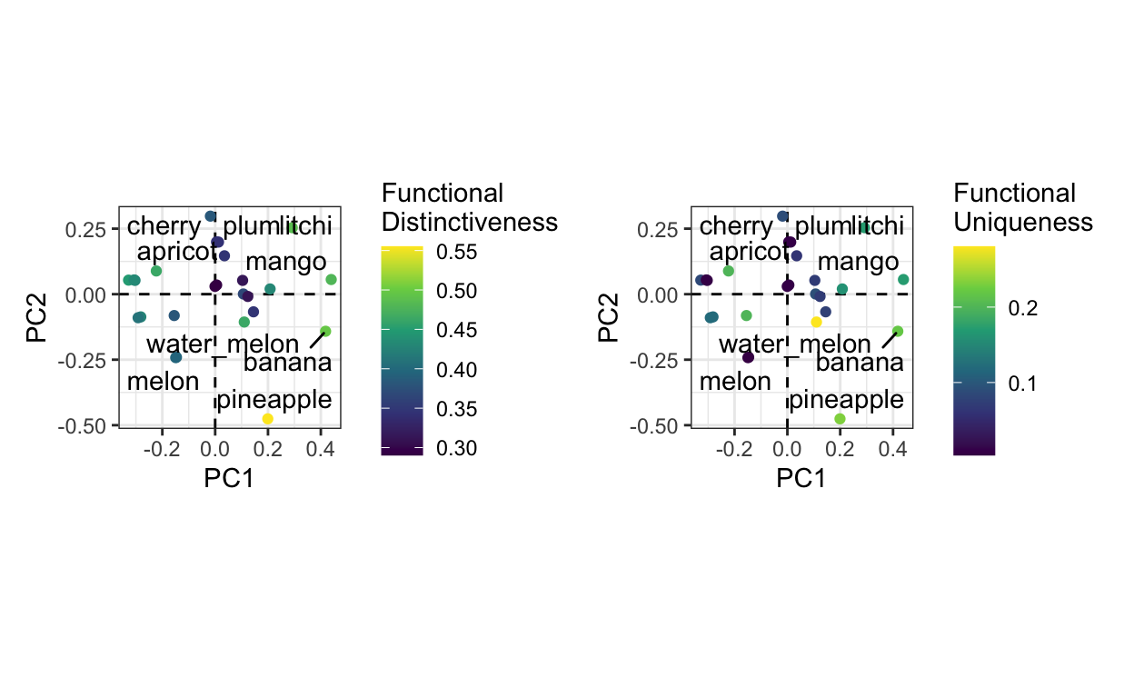
We can clearly see that, by definition, most functionally distinct species are on the edges of the functional space (pineapple, litchi, mango). If we compare both plots, we realize that functional distinctiveness doesn’t always come with functional uniqueness. One strange observation is that passion-fruit has a very functional uniqueness even though it seems quite in the middle of the points. This is a consequence of using the raw trait dissimilarity matrix instead of the projected axes. We’re are here visualizing the position of passion fruit in a 2D space while it should be considered in a 5D space, so it may seem close to other points in 2D while it is further away in reality.

As was done with mFD to correlate the functional axes with species’ traits we can correlate functional distinctiveness to specific traits in order to see which traits are mainly driving distinctiveness.

Regarding local level functional originality indices, the visualization can be more difficult to grasp and depends highly on the question. Would you rather focus on visualizing the functional distinctiveness of one species across communities? Compare the distribution of functional distinctiveness values across communities?

One idea to keep in mind is that averaging functional distinctiveness per community is exactly equal to computing functional dispersion. Functional originality is computed on a species basis, so we should be aware that if we are rather interested by community properties than we can compute functional diversity metrics which are much more appropriate.

If we take again our example of the apple we can see to what extent its functional distinctiveness varies across baskets compared to lemon.

local_di_ap <- as.data.frame(sp_local_di[, c(1, 11)])
local_di_ap$basket <- rownames(local_di_ap)

You can of course then compute relationship between environmental covariates and functional originality values. Because we don’t have any covariable in our fruit baskets we will stop the plotting session here.

3.4.2 Plotting rarity

We can plot also the rarity indices we computed and compared them to the functional rarity indices.

sp_di_ri <- merge(sp_di, ri, by = "species")
sp_di_ri_ui <- merge(sp_di_ri, sp_ui, by = "species")

plot_dist_ri_reg <- ggplot(sp_di_ri, aes(distinctiveness, Ri)) +
  geom_point() +
  ggrepel::geom_text_repel(aes(label = species)) +
  labs(x = "Functional Distinctiveness", y = "Geographical Restrictedness") +
  theme_bw() +
  theme(aspect.ratio = 1)

plot_dist_ri_reg

On this visualization we can clearly see that pineapple is overall the most distinct species while being quite restricted in terms of baskets. On the other hand, apple is the most functionally common and regionally widespread fruit (low restrictedness).

We can produce similar plot with functional uniqueness:

plot_ui_ri_reg <- ggplot(sp_di_ri_ui, aes(Ui, Ri)) +
  geom_point() +
  ggrepel::geom_text_repel(aes(label = species)) +
  labs(x = "Functional Uniqueness", y = "Geographical Restrictedness") +
  theme_bw() +
  theme(aspect.ratio = 1)

plot_ui_ri_reg

We observe a rather similar plot for functional uniqueness than for functional distinctiveness.

We can also try to plot local scale measurements. We first convert the full matrix of indices into easier to work with data frames through the matrix_to_stack() function.

sp_local_di_df <- matrix_to_stack(
  sp_local_di, value_col = "local_di", row_to_col = "basket",
  col_to_col = "species"
)
sp_local_si_df <- matrix_to_stack(
  si, value_col = "local_si", row_to_col = "basket", col_to_col = "species"
)

sp_local_di_si <- merge(
  sp_local_di_df, sp_local_si_df, by = c("basket", "species")
)

head(sp_local_di_si)

    basket       species  local_di  local_si
1 basket_1         apple 0.1977721 0.3298770
2 basket_1        banana 0.4642749 0.7578583
3 basket_1        cherry 0.3491350 0.6597540
4 basket_1         lemon 0.3042315 0.5743492
5 basket_1         melon 0.3334516 0.5743492
6 basket_1 passion_fruit 0.4899472 0.7578583

Now that we have properly formatted data we can make our local plot.

plot_local_di_si <- ggplot(sp_local_di_si, aes(local_di, local_si)) +
  geom_point(alpha = 1/3) +
  labs(x = "Functional Distinctiveness", y = "Scarcity") +
  theme_bw() +
  theme(aspect.ratio = 1)

plot_local_di_si

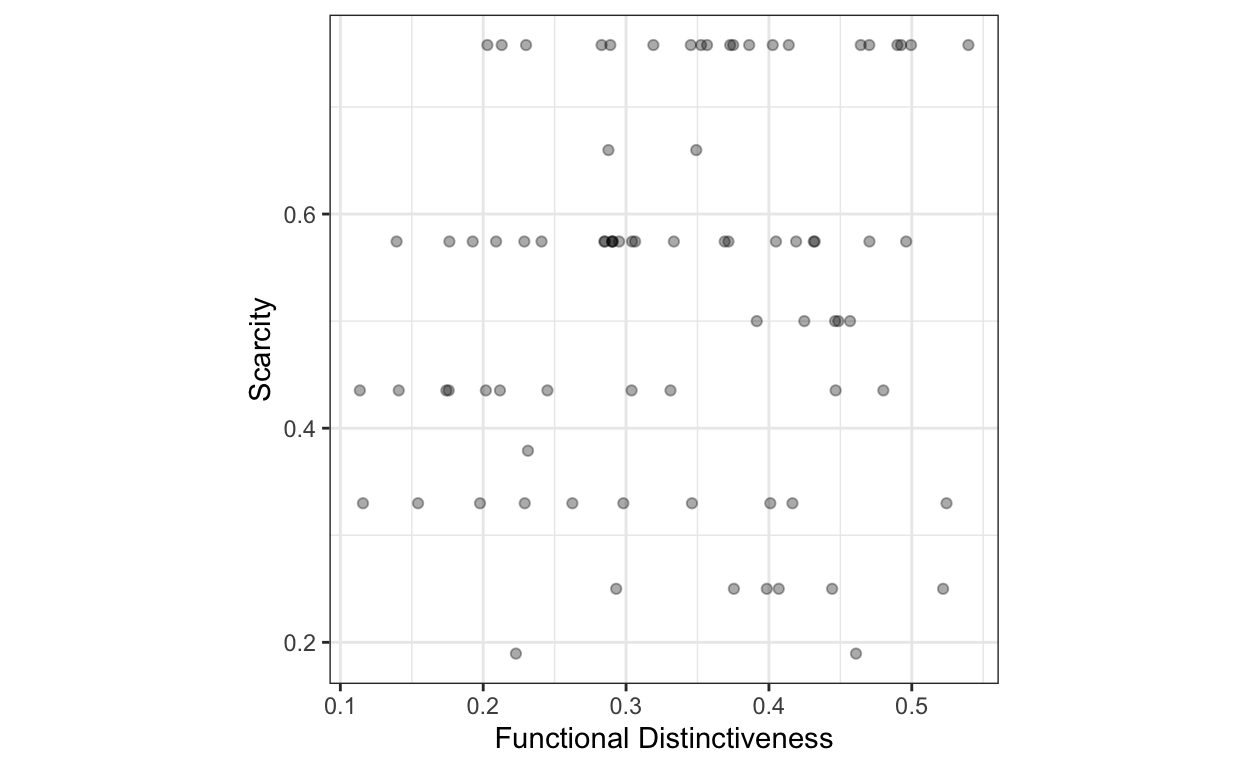
There seems to be no correlation between functional distinctiveness and scarcity. So locally rare fruits are not necessarily distinct.

That plot concludes our plotting section on functional rarity indices.

Corrections

If you see mistakes or want to suggest changes, please Create an issue on the source repository.

Reuse

The material of this website is licensed under Creative Commons Attribution CC BY 4.0. Source code is available at https://github.com/frbcesab/workshop-free/.

Citation

Casajus N, Grenié M, Magneville C & Villéger S (2022) Workshop FRB-CESAB & FREE Working Group: Functional Rarity and Diversity in Ecology.

Practice

About

Prerequisites

Data description

Questions

Part 1. Build a functional space using the mFD package

1.0. Compute summaries about your data

1.1. What about the traits?

1.2. Computing distances between species based on functional traits

1.3. Building functional spaces and chosing the best one

1.3.1. Computing several multimensional functional spaces and assessing their quality

1.3.2. Illustrating the quality of the functional spaces

1.3.3. Testing the correlation between functional axes and traits

1.4. Plotting the selected functional space and position of species

Part 2. Computing and plotting FD indices using the mFD package

2.1. Computing and plotting alpha FD indices

2.2. Computing and plotting beta FD indices

Part 3. Functional rarity

3.1 Components of functional rarity: trait originality and rarity

3.2 Different indices of functional rarity

3.2.1 Functional originality indices

3.2.1 Rarity indices indices

3.3 Computing functional rarity

3.3.1 Functional originality at regional scale

3.3.2 Functional originality at local scale

3.3.3 Rarity indices

3.4 Plotting functional rarity

3.4.1 Plotting functional originality

3.4.2 Plotting rarity

Corrections

Reuse

Citation

Part 1. Build a functional space using the `mFD` package

Part 2. Computing and plotting FD indices using the `mFD` package