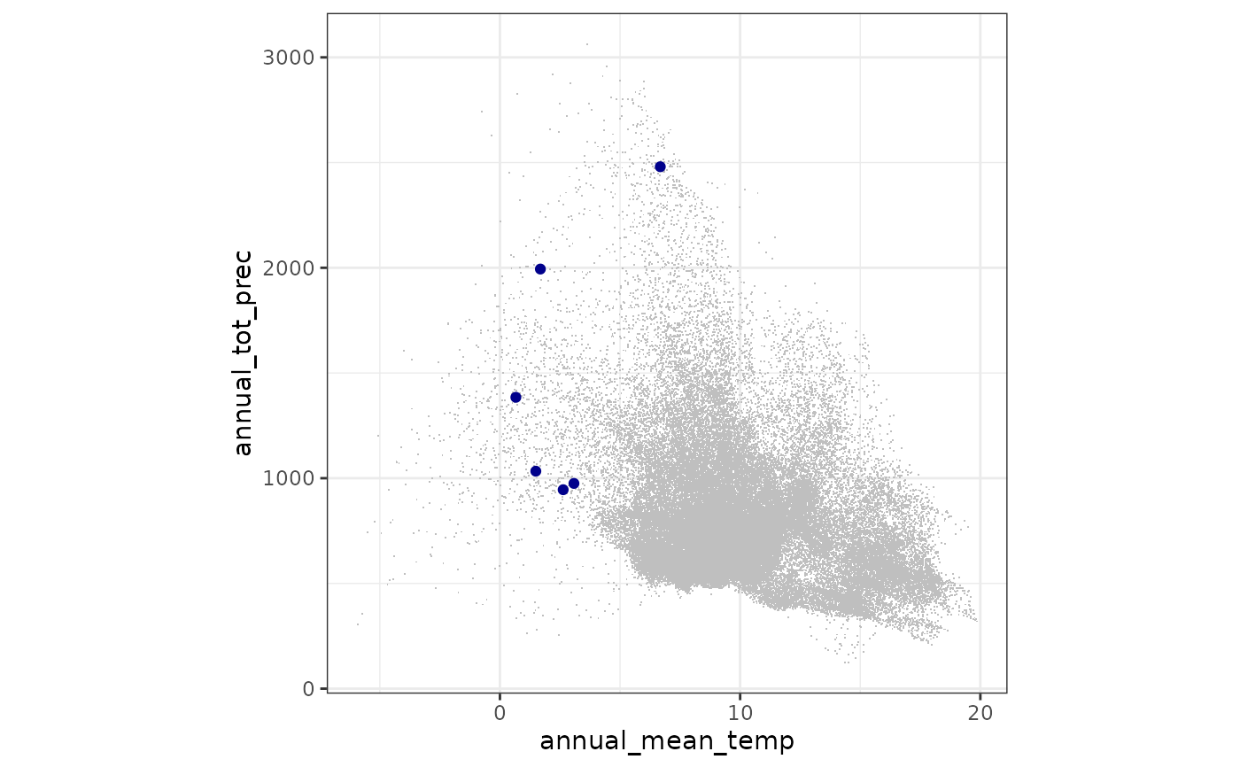
Plot Position of Sites in Environmental Space — fb_plot_site

Plot a figure showing the average environmental space of given sites compared to a full environmental vector. For the sake of simplicity only represents the figure along two environmental axes. The average environmental value are extracted for each site.

Usage

fb_plot_site_environment(
  site_locations,
  environment_raster,
  first_layer = names(environment_raster)[1],
  second_layer = names(environment_raster)[2]
)

Arguments

site_locations: an sf object with the spatial geometries of sites. NOTE: the first column should be named "site" and indicate site names.
environment_raster: a SpatRaster object (package terra). A single or multi-layers environmental raster.
first_layer: character(1) the name of the first layer to use, by default uses the first layer of environment_raster
second_layer: character(1) the name of the second layer to use, by default uses the second layer of environment_raster

Value

a ggplot object

Examples

data("site_locations")

# Import climate rasters
prec <- system.file("extdata", "annual_tot_prec.tif", package = "funbiogeo")
tavg <- system.file("extdata", "annual_mean_temp.tif", package = "funbiogeo")

layers <- terra::rast(c(tavg, prec))

# Make plot (show environmental position of 6 first sites)
fb_plot_site_environment(head(site_locations), layers)
#> Warning: Removed 49503 rows containing missing values or values outside the scale range
#> (`geom_point()`).