funbiogeo provides an easy way to upscale your site’s
data to a coarser resolution. The idea is that you have any type of data
at the site level (diversity metrics, environmental data, as well as
site-species data) that you would like to work on or visualize on a
coarser scale. The aggregation process can look daunting at first and be
quite difficult to run. We explain in detail, throughout this vignette,
how to do so with the fb_aggregate_site_data() function.
We’ll detail three use cases:
- Aggregating through a regular square grid
- Aggregating to irregular polygons (like countries, biomes, or any other shape )
- Aggregating using a raster grid
In all three cases, the aggregation can work on any data available at the site-level. This could be species richness, site-species data, or functional diversity metrics.
Preamble: Getting Site-Level Data
library("funbiogeo")
library("sf")
#> Linking to GEOS 3.12.1, GDAL 3.8.4, PROJ 9.4.0; sf_use_s2() is TRUE
library("ggplot2")
Let’s import our site by locations object, which describes the geographical locations of sites.
data("woodiv_locations")

woodiv_locations
#> Simple feature collection with 5366 features and 2 fields
#> Geometry type: POLYGON
#> Dimension:     XY
#> Bounding box:  xmin: 2630000 ymin: 1380000 xmax: 5040000 ymax: 2550000
#> Projected CRS: ETRS89-extended / LAEA Europe
#> First 10 features:
#>        site  country                       geometry
#> 1  26351755 Portugal POLYGON ((2630000 1750000, ...
#> 2  26351765 Portugal POLYGON ((2630000 1760000, ...
#> 4  26351955 Portugal POLYGON ((2630000 1950000, ...
#> 5  26351965 Portugal POLYGON ((2630000 1960000, ...
#> 6  26451755 Portugal POLYGON ((2640000 1750000, ...
#> 7  26451765 Portugal POLYGON ((2640000 1760000, ...
#> 8  26451775 Portugal POLYGON ((2640000 1770000, ...
#> 10 26451955 Portugal POLYGON ((2640000 1950000, ...
#> 11 26451965 Portugal POLYGON ((2640000 1960000, ...
#> 12 26451975 Portugal POLYGON ((2640000 1970000, ...
These sites are a collection of regular spatial polygons at a
resolution of 10 km x 10 km over South Western Europe. Our site by
locations object is a sf object, which means it’s a spatial
object coupled with a data.frame.
For each site, we want to compute the species richness. We can do so
by counting the species at each site with the function
fb_count_species_by_site().
# Import site x species data
data("woodiv_site_species")

# Compute species richness
species_richness <- fb_count_species_by_site(woodiv_site_species)

head(species_richness)
#>       site n_species  coverage
#> 1 40552295        12 0.5000000
#> 2 39252405        12 0.5000000
#> 3 37752305        12 0.5000000
#> 4 39852255        12 0.5000000
#> 5 39152415        12 0.5000000
#> 6 39552415        11 0.4583333
Unfortunately, the fb_count_species_by_site() doesn’t
output a spatial object but a data.frame with three columns: the
identifier of the site, the number of species, and the proportion of
species present at a given site. Before going any further, let’s put
species richness on the map with the function
fb_map_site_data(). That function allows us to represent
any arbitrary data at the site level by combining it with the site by
locations object, and it shows a map of that data:
fb_map_site_data(woodiv_locations, species_richness, "n_species")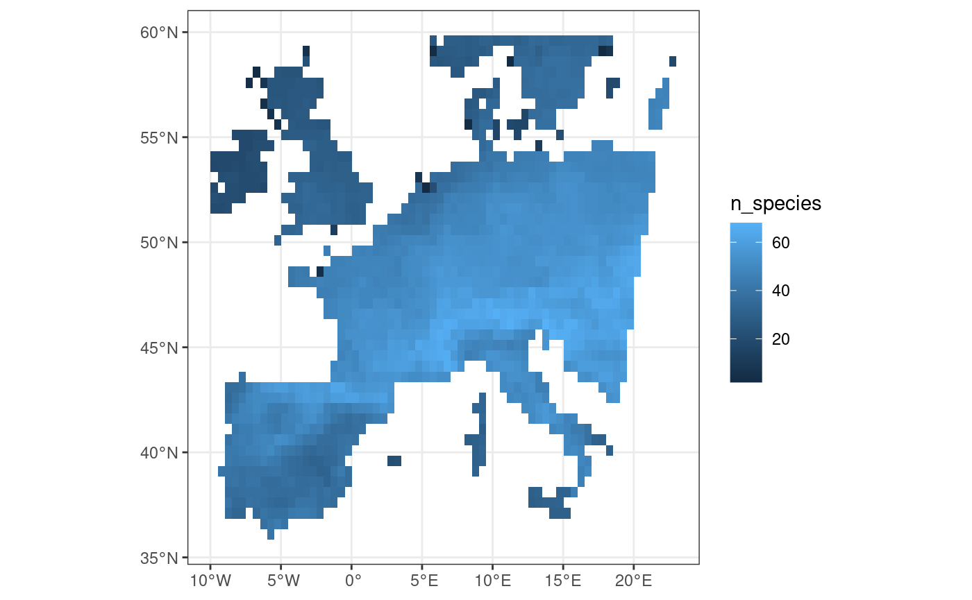
Now, from this site-level species richness, we would like to get
species richness at different scales. First, we’ll show how to aggregate
on a coarser square grid, then at the country level, and then with a
grid from a SpatRaster.
Aggregating Through a Square Grid
Our initial sites are 10km by 10km, we want to aggregate using a grid
with pixels of 300km by 300km. When aggregating with a such a grid,
there are two possibilities: either you already have a defined grid as a
spatial object or you generate one on the fly. Here we’ll generate the
grid on the fly using the function st_make_grid() from the
sf package.
Because our data are using a map projection
with units in meters, we can directly specify the cellsize
argument of st_make_grid(). The function the locations
object as the first argument, then a vector of two numbers as the second
argument defining the cell sizes. By default, the newly created grid
will cover the same extent as in the input spatial data.
coarser_grid <- sf::st_make_grid(woodiv_locations, cellsize = c(300e3, 300e3))

head(coarser_grid)
#> Geometry set for 6 features
#> Geometry type: POLYGON
#> Dimension:     XY
#> Bounding box:  xmin: 2630000 ymin: 1380000 xmax: 4430000 ymax: 1680000
#> Projected CRS: ETRS89-extended / LAEA Europe
#> First 5 geometries:
#> POLYGON ((2630000 1380000, 2930000 1380000, 293...
#> POLYGON ((2930000 1380000, 3230000 1380000, 323...
#> POLYGON ((3230000 1380000, 3530000 1380000, 353...
#> POLYGON ((3530000 1380000, 3830000 1380000, 383...
#> POLYGON ((3830000 1380000, 4130000 1380000, 413...
Because the coarser grid is a sfc object, we need to
transform it into a sf object to be fully compatible with
fb_aggregate_site_data(). We do so in the next chunk:
coarser_grid <- sf::st_as_sf(coarser_grid)

coarser_grid
#> Simple feature collection with 36 features and 0 fields
#> Geometry type: POLYGON
#> Dimension:     XY
#> Bounding box:  xmin: 2630000 ymin: 1380000 xmax: 5330000 ymax: 2580000
#> Projected CRS: ETRS89-extended / LAEA Europe
#> First 10 features:
#>                                 x
#> 1  POLYGON ((2630000 1380000, ...
#> 2  POLYGON ((2930000 1380000, ...
#> 3  POLYGON ((3230000 1380000, ...
#> 4  POLYGON ((3530000 1380000, ...
#> 5  POLYGON ((3830000 1380000, ...
#> 6  POLYGON ((4130000 1380000, ...
#> 7  POLYGON ((4430000 1380000, ...
#> 8  POLYGON ((4730000 1380000, ...
#> 9  POLYGON ((5030000 1380000, ...
#> 10 POLYGON ((2630000 1680000, ...
Now that we have a new grid, we can plot it with the original site
locations data to make sure it is sensible, compared to what we wanted.
We will do so using the geom_sf() function from
ggplot2.
ggplot() +
  geom_sf(data = coarser_grid, aes(fill = "coarser")) +
  geom_sf(data = woodiv_locations, aes(fill = "original")) +
  # Color the grids
  scale_fill_manual(
    values = c(original = "darkorange", coarser = "darkmagenta")
  ) +
  theme_bw()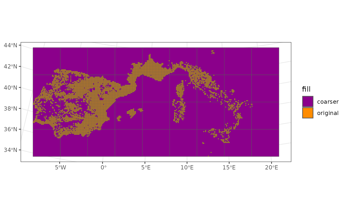
In orange, you see the original data grid of the data, while in purple is the coarser grid we defined over which we’ll aggregate the data.
We’re interested in knowing the occurrence of our Mediterranean plant
species over each pixel of the coarser grid. To do this, we’ll use the
fb_aggregate_site_data() function from
funbiogeo. It takes as first argument the site-locations
object (including the column with the site ids), then the data that
needs to be aggregated (with the site ids column), then the grid over
which to aggregate the data, finally, the last argument is the function
to use to aggregate the data. By default, uses the mean()
function and assumes quantitative site data only.
Because we’re interested in species richness, we’ll use the dataset
we computed in the first section, which defines species richness at each
site. We’ll use the fb_aggregate_site_data() function on
our original site-locations object, with the species richness data, on
the coarser grid, using the mean() function to get back the
average species richness across sites per larger pixel.
coarser_richness <- fb_aggregate_site_data(
  woodiv_locations,
  species_richness,
  coarser_grid,
  fun = mean
)

head(coarser_richness)
#> Simple feature collection with 6 features and 2 fields
#> Geometry type: POLYGON
#> Dimension:     XY
#> Bounding box:  xmin: 2630000 ymin: 1380000 xmax: 4430000 ymax: 1680000
#> Projected CRS: ETRS89-extended / LAEA Europe
#>   n_species   coverage                       geometry
#> 1  1.700000 0.07083333 POLYGON ((2630000 1380000, ...
#> 2  2.690821 0.11211755 POLYGON ((2930000 1380000, ...
#> 3  1.795918 0.07482993 POLYGON ((3230000 1380000, ...
#> 4        NA         NA POLYGON ((3530000 1380000, ...
#> 5        NA         NA POLYGON ((3830000 1380000, ...
#> 6        NA         NA POLYGON ((4130000 1380000, ...
Note that the object we obtain is also a sf object of
the same type as the grid we provided.
We can plot it using ggplot2:
ggplot(coarser_richness, aes(fill = n_species)) +
  geom_sf() +
  scale_fill_viridis_c() +
  theme_bw()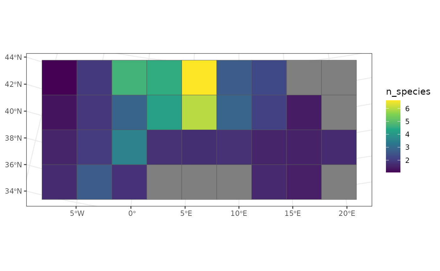
We see that the pixels of the North show the greatest average species richness, especially in the South of France.
Aggregating Through Irregular Polygons
We aggregated our richness data on a regular grid with square pixels,
but it is very common in biogeography to want to aggregate data on
spatial objects that are of irregular shapes. For example, aggregating
data at the biome or the country scale. Initially, our data may be on a
regular grid, but we want to aggregate at the country scale. This is
easily doable with the fb_aggregate_site_data()
function.
The function actually works with any arbitrary sf object
as an aggregation grid whether it’s polygons regular or not, lines,
points, or a mix of any geometries.
To show you how to do it, we’ll use the included spatial object for the four Mediterrannean countries covered by our example dataset:
# Load the file from the package folder
countries <- readRDS(
  system.file("extdata", "countries_sf.rds", package = "funbiogeo")
)

# Visualize the spatial object
ggplot(countries) +
  geom_sf(aes(fill = name)) +
  geom_sf(data = woodiv_locations, alpha = 1 / 2) + # Add original data
  geom_sf_text(aes(label = name)) +
  theme_bw()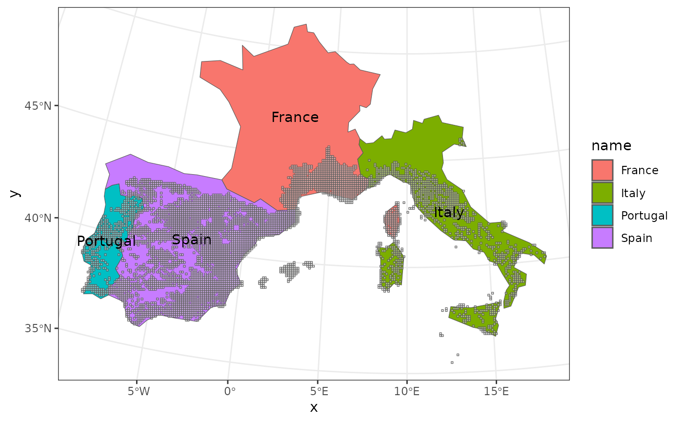
As we already have our aggregation object, here the countries’
delimitation, we can directly use the
fb_aggregate_site_data() function on: the original
locations, the species richness data, and the countries object, with the
mean() function. As such, we’ll obtain the average species
richness in Mediterrannean tree species per country. Note that all the
sites that are not covered by the aggregation polygons (here the
countries) are going to be dropped.
# Compute country-level average species richness
countries_richness <- fb_aggregate_site_data(
  woodiv_locations,
  species_richness,
  countries,
  fun = mean
)

# Map country-level average species richness
ggplot(countries_richness) +
  geom_sf(aes(fill = n_species)) +
  theme_bw()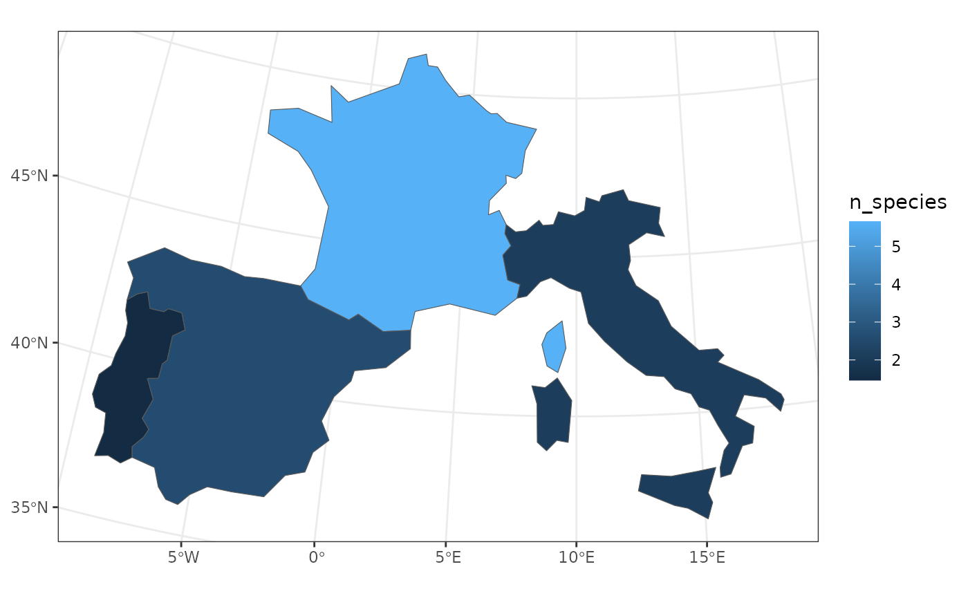
We observe that France has a higher species richness than other countries, with more than 5 species on average in the sites it harbors.
Aggregating Through a SpatRaster Grid
In the two previous sections, we saw how to aggregate on arbitrary shaped polygons. However, another quite common use case, especially when working with species distribution model, is to want to aggregate data follow an environmental raster or a raster grid.
We would now like to aggregate our sites at the same resolution as is
available for our environmental data such as mean annual temperature. We
need to aggregate site data on a SpatRaster spatial grid
(from the terra
package). A nice property of fb_aggregate_site_data()
function is that it outputs a matching type of object as the provided
grid. If it’s a sf object, then the function will output
the same type of sf object, while if it’s a
SpatRaster then it will give back a SpatRaster
object.
First of all, we can create a coarser grid based on our location object.
# Import study area grid
coarser_grid <- system.file("extdata", "grid_area.tif", package = "funbiogeo")
coarser_grid <- terra::rast(coarser_grid)

coarser_grid
#> class       : SpatRaster
#> size        : 29, 41, 1  (nrow, ncol, nlyr)
#> resolution  : 0.8333333, 0.8333333  (x, y)
#> extent      : -10.5, 23.66667, 35.83333, 60  (xmin, xmax, ymin, ymax)
#> coord. ref. : lon/lat WGS 84 (EPSG:4326)
#> source      : grid_area.tif
#> name        : value
#> min value   :     1
#> max value   :     1
We will aggregate the site data (resolution of 10 km by 10 km) to
this new coarser raster (resolution of 0.83°, close to 92 km by 92km)
with the function fb_aggregate_site_data(). This function
requires the following arguments:
-
site_locations: the site x locations object -
site_data: amatrixordata.framecontaining values per site to aggregate on the provided gridagg_geom. Can have one or several columns (variables to aggregate). The first column must contain site names as provided in the objectspecies_richness -
agg_geom: aSpatRasterobject (packageterra). A raster of one single layer that defines the grid along which to aggregate. -
fun: the function used to aggregate site values when there are multiple sites in one cell (do we want to get the minimum value? the maximum? the sum? Or the mean?)
Let’s compute our average species richness values across our grid.
# Upscale to grid ----
upscaled_richness <- fb_aggregate_site_data(
  site_locations = woodiv_locations[, 1, drop = FALSE],
  site_data = species_richness[, 1:2],
  agg_geom = coarser_grid,
  fun = mean
)

upscaled_richness
#> class       : SpatRaster
#> size        : 29, 41, 1  (nrow, ncol, nlyr)
#> resolution  : 0.8333333, 0.8333333  (x, y)
#> extent      : -10.5, 23.66667, 35.83333, 60  (xmin, xmax, ymin, ymax)
#> coord. ref. : lon/lat WGS 84 (EPSG:4326)
#> source(s)   : memory
#> varname     : grid_area
#> name        : n_species
#> min value   :         1
#> max value   :        10
We get a SpatRaster object that is of the same
resolution as our provided agg_geom raster grid. The cells
of this raster contain the averaged values of species richness of our
sites aggregated on the coarser grid. We can plot these values through a
call to fb_map_raster() which allows to plot rasters.
fb_map_raster(upscaled_richness)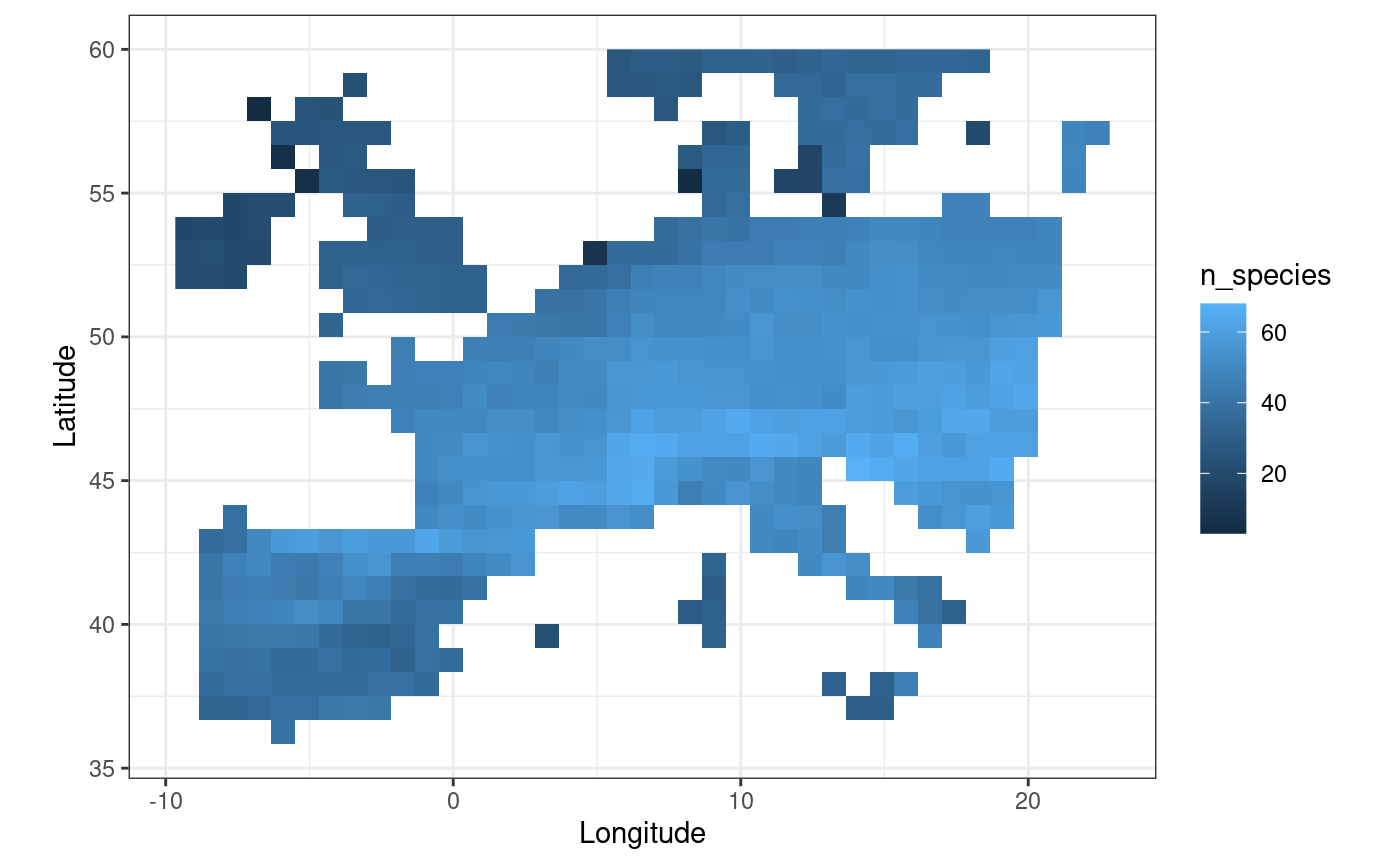
Specific Examples
Coarsening Site x Species Data
Through the fb_aggregate_site_data() function, we can
also coarsen our site-species grid by selecting the appropriate function
as the fun argument, we detail how in this section.
Now that we’ve learned how to aggregate arbitrary data at the site
scale over a spatial scale. We’re going to use our provided example
named site_species at a resolution of 10 x 10 km to get new
sites from a grid with pixels of 0.83° of resolution.
As shown in the previous section, we’ll need three objects:
site_species, which describes the species present across
sites; site_locations, which gives the spatial locations of
sites; and agg_geom which is a SpatRaster
object defining the coarser grid.
We’ll use the previously defined object to run our example. To
aggregate the presence-absence of species within each pixel of the new
grid, we’ll use the max() function (as the fun
argument). As such, coarser pixels, which contain a mix of presence and
absence of certain species, we’ll be considered as having the species
present. Only when the species is absent from all of the finer scale
sites, will the coarser pixels show the species as absent.
site_species_agg <- fb_aggregate_site_data(
  woodiv_locations[, 1, drop = FALSE],
  woodiv_site_species,
  agg_geom = coarser_grid,
  fun = max
)
The returned object is a SpatRaster as well but can be
easily transformed into a data.frame to follow back with the regular
analyses provided in funbiogeo. The new object contains one
layer for each aggregated variable, i.e., here, one per species.
site_species_agg
#> class       : SpatRaster
#> size        : 29, 41, 24  (nrow, ncol, nlyr)
#> resolution  : 0.8333333, 0.8333333  (x, y)
#> extent      : -10.5, 23.66667, 35.83333, 60  (xmin, xmax, ymin, ymax)
#> coord. ref. : lon/lat WGS 84 (EPSG:4326)
#> source(s)   : memory
#> varnames    : grid_area
#>               grid_area
#>               grid_area
#>               grid_area
#>               grid_area
#>               ...
#> names       : AALB, ACEP, APIN, CLIB, CSEM, JCOM, ...
#> min values  :    0,    0,    0,    0,    0,    0, ...
#> max values  :    1,    1,    1,    0,    1,    1, ...
We can visualize both maps for a single species to see the difference in resolution :
single_species <- merge(
  woodiv_locations,
  woodiv_site_species[, 1:2],
  by = "site",
  all = TRUE
)

finer_map <- ggplot(single_species) +
  geom_sf(aes(fill = as.factor(AALB))) +
  labs(fill = "Presence of AALB", title = "Original resolution (10 x 10 km)")

coarser_map <- fb_map_raster(site_species_agg[[1]]) +
  scale_fill_binned(breaks = c(0, 0.5, 1)) +
  labs(title = "Coarser resolution (0.83°)")

patchwork::wrap_plots(finer_map, coarser_map, nrow = 1)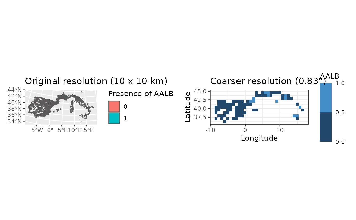
Obtaining Back a Site x Species data.frame
Now we have obtained a raster of aggregated site-species presences.
However, the other functions of funbiogeo don’t play well
with raster data. They need data.frames to work well. We can do this
through the specific function as.data.frame() in
terra (make sure to check the dedicated help page that
specifies all the additional arguments with
?terra::as.data.frame).
# Use the 'cells = TRUE' argument to index results with a new cell column
# corresponding to the ID of the coarser grid pixels
site_species_agg_df <- terra::as.data.frame(site_species_agg, cells = TRUE)

site_species_agg_df[1:4, 1:4]
#>     cell AALB ACEP APIN
#> 755  755    0    0    0
#> 757  757    0    0    1
#> 758  758    1    0    0
#> 759  759    1    0    0

colnames(site_species_agg_df)[1] <- "site"
With this, we’re ready to reuse all of funbiogeo
functions to work on these coarser data. You can proceed similarly to
aggregate the ancillary site-related data, to use them in the rest of
the analyses.
Upscaling Functional Diversity Data
Because funbiogeo focuses on the functional biogeography
workflow, we’ll explore in this section how to aggregate the results for
a functional biogeography function. First, we’ll detail an example
aggregating the community-weighted mean (CWM) of plant height, which is
the abundance-weighted trait average of the assemblage. Second, we’ll
show an example of coarsing functional diversity metrics computed
through the fundiversity
package.
Coarsen CWM of Plant Height
To compute the CWM we’ll use the function fb_cwm().
site_cwm <- fb_cwm(woodiv_site_species, woodiv_traits[, 1:2])

head(site_cwm)
#>       site        trait      cwm
#> 1 26351755 plant_height 12.31767
#> 2 26351765 plant_height  4.88150
#> 3 26351955 plant_height 12.31767
#> 4 26351965 plant_height 13.77575
#> 5 26451755 plant_height  4.88150
#> 6 26451765 plant_height 15.76845
Now we can aggregate the CWM of plant height at a coarser scale using
fb_aggregate_site_data() as done in the previous sections,
this time using the default fun argument, as we want to
compute the average CWM:
colnames(site_cwm)[3] <- "plant_height"

upscaled_cwm <- fb_aggregate_site_data(
  woodiv_locations[, 1, drop = FALSE],
  site_cwm[, c(1, 3)],
  coarser_grid
)

upscaled_cwm
#> class       : SpatRaster
#> size        : 29, 41, 1  (nrow, ncol, nlyr)
#> resolution  : 0.8333333, 0.8333333  (x, y)
#> extent      : -10.5, 23.66667, 35.83333, 60  (xmin, xmax, ymin, ymax)
#> coord. ref. : lon/lat WGS 84 (EPSG:4326)
#> source(s)   : memory
#> varname     : grid_area
#> name        : plant_height
#> min value   :       4.8815
#> max value   :    42.143066
We can then map the CWM using the fb_map_raster()
function:
fb_map_raster(upscaled_cwm) +
  scale_fill_continuous(trans = "log10")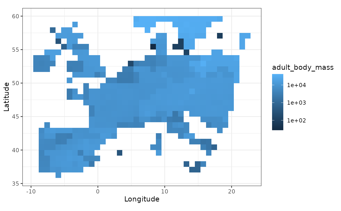
Coarser FRic Through fundiversity
In a similar fashion as in the introduction
vignette to funbiogeo in this section, we’ll compute
the Functional Richness using two traits across our example dataset.
# Get all species for which we have both adult body mass and litter size
subset_traits <- woodiv_traits[,
  c("species", "plant_height", "seed_mass")
]
subset_traits <- subset(
  subset_traits,
  !is.na(plant_height) & !is.na(seed_mass)
)

# Transform trait data
subset_traits[["plant_height"]] <- as.numeric(
  scale(log10(subset_traits[["plant_height"]]))
)

subset_traits[["seed_mass"]] <- as.numeric(
  scale(subset_traits[["seed_mass"]])
)

# Filter site for which we have trait information for than 80% of species
subset_site <- fb_filter_sites_by_trait_coverage(
  woodiv_site_species,
  subset_traits,
  0.8
)

subset_site <- subset_site[, c("site", subset_traits$species)]

# Remove first column and convert in rownames
rownames(subset_traits) <- subset_traits[["species"]]
subset_traits <- subset_traits[, -1]

rownames(subset_site) <- subset_site[["site"]]
subset_site <- subset_site[, -1]

# Compute FRic
site_fric <- fundiversity::fd_fric(
  subset_traits,
  subset_site
)
#> Warning in fundiversity::fd_fric(subset_traits, subset_site): Some sites had
#> less species than traits so returned FRic is 'NA'

head(site_fric)
#>       site      FRic
#> 1 41152325 1.0964687
#> 2 40852325 1.1380385
#> 3 40852345 1.1523280
#> 4 42552105 0.8201878
#> 5 41152315 1.1380385
#> 6 37452365        NA
We can now follow a similar upscaling process as in the previous sections to compute the average functional richness on a coarser spatial scale:
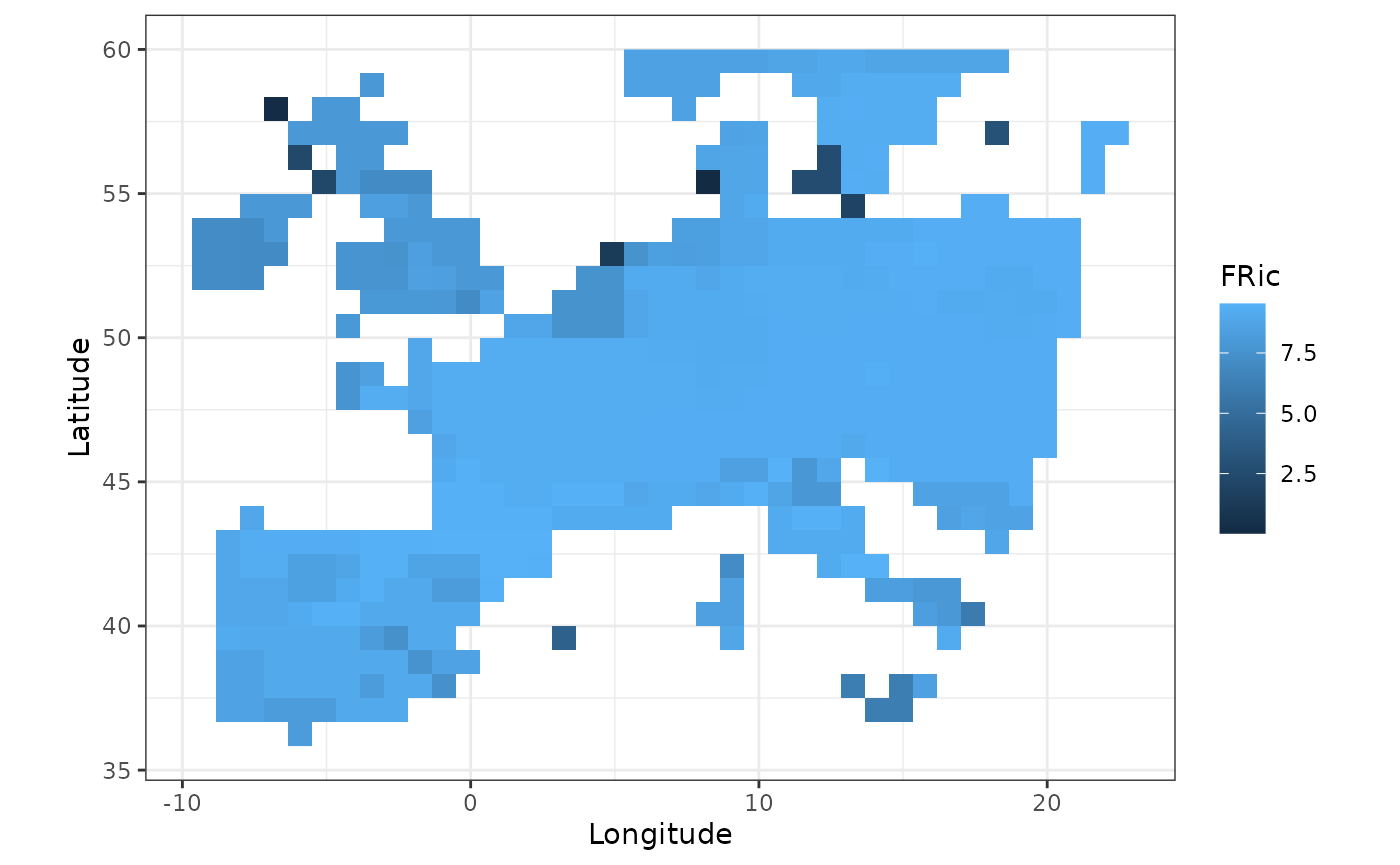
agg_fric <- fb_aggregate_site_data(
  woodiv_locations[, 1, drop = FALSE],
  site_fric,
  coarser_grid
)

fb_map_raster(agg_fric)
#> Warning: Raster pixels are placed at uneven horizontal intervals and will be shifted
#> ℹ Consider using `geom_tile()` instead.