suppressPackageStartupMessages({
library(mapview)
library(here)
library(sf)
library(terra)
})Lines
ImportantSummary
This tutorial explores how to handle spatial lines in with terra package:
- load a spatial object with
terra::vect() - calculate length of lines with
terra::perim() - calculate distances between points and lines with
terra::distance()
TipThe ecologist mind
Otters live along rivers, but how far from the rivers were they observed? To answer this question, we will need to discover another type of vector: lines.
Setup
Follow the setup instructions if you haven’t followed the tutorial on points
If haven’t done it already, please follow the setup instructions. Let’s start with loading the required packages.
pt_otter <- vect(here("data", "gbif_otter_2021_mpl50km.gpkg"))pt_otter <- vect(
"https://github.com/FRBCesab/spatial-r/raw/main/data/gbif_otter_2021_mpl50km.gpkg"
)Load lines from a geopackage file
Lines are made of multiple points. It is possible to create lines directly from coordinates but, in practice, it often comes from an existing spatial dataset. In our example, we will load rivers for the area of interest from IGN data BD CARTO.
Note that this dataset has rough resolution (BD TOPO would be recommended for real analysis), but it’s perfect for our illustration and learning purpose.
You can load vector data with the function terra::vect().
river <- vect(here("data", "BDCARTO-River_mpl50km.gpkg"))In sf, there are two functions to read vector data sf::st_read() and sf::read_sf(). The main difference lies in the format of the attribute table: it is stored as data.frame with st_read, and as a tibble with read_sf().
river_sf <- st_read(here("data", "BDCARTO-River_mpl50km.gpkg"))Reading layer `BDCARTO-River_mpl50km' from data source
`/home/romain/GitHub/spatial-r/data/BDCARTO-River_mpl50km.gpkg'
using driver `GPKG'
Simple feature collection with 2110 features and 8 fields
Geometry type: MULTILINESTRING
Dimension: XY
Bounding box: xmin: 3.18983 ymin: 43.21278 xmax: 4.56447 ymax: 44.16754
Geodetic CRS: WGS 84If you don’t have the data locally (and won’t use it repeatedly), you can load it directly with:
river <- vect(
"https://github.com/FRBCesab/spatial-r/raw/refs/heads/main/data/BDCARTO-River_mpl50km.gpkg"
)
NoteYour turn
- How many different stretches of river was loaded?
- What is the coordinate reference system (CRS) of the loaded river data?
- Can you get the name of the all the river stretches?
Click to see the answer
- There are
2110stretches (=lines) in the dataset. You can access it withdim(river),nrow(river)or just by typingriverin the console.
- The coordinates are in
WGS 84(EPSG4326). You can access this information withcrs(river, describe = TRUE)(or insfwithst_crs(river_sf)). - The column that stored the name of river stretches is
toponyme. You could identify it withhead(river)ornames(river). There are151river stretches without names (table(is.na(river$toponyme))).
Calculate length of lines
TipThe ecologist mind
Can we see whether otters were observed close to small or large rivers? We will approximate the rivers’ size by their length.
When calculating distances and length, be careful with projection systems. Some are not suited to calculate distance, prefer equidistance projections or use local projection systems. Recent implementation of terra and sf calculates spherical distances when using geographic coordinates (in longitude and latitude) which is the most accurate and recommended to account for Earth’s curvature.
The function terra::perim() returns the length of lines in meters.
# calculate the length of rivers (in km)
river$length_km <- perim(river) / 1000The function sf::st_length() calculate the length of lines.
# calculate the length of rivers (in km)
river_sf$length_km <- st_length(river_sf) / 1000# see the distribution of river length
boxplot(river$length_km, ylab = "length (km)")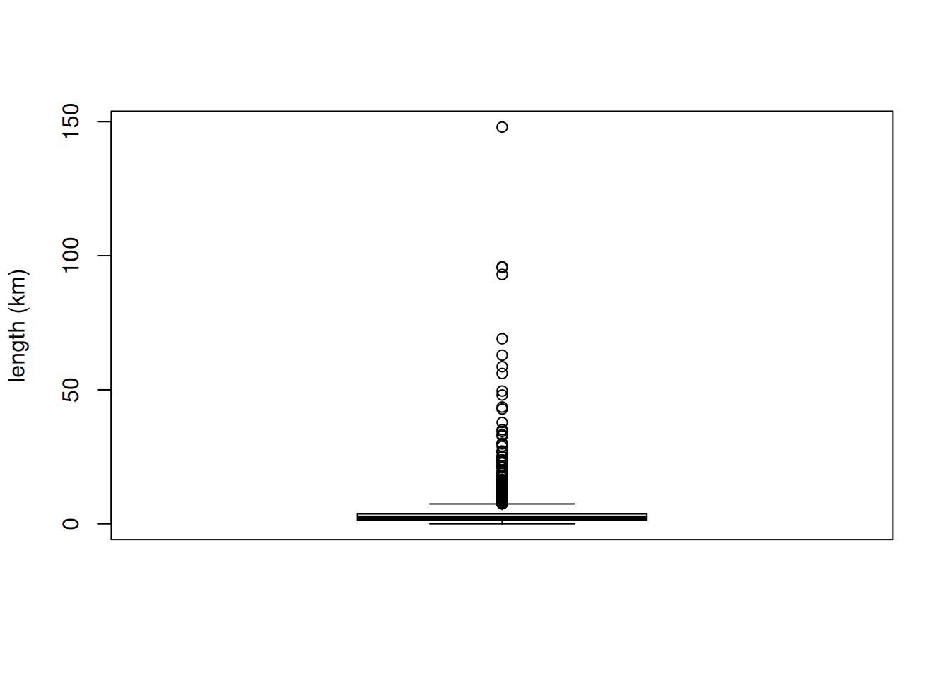
NoteYour turn
- Which is the longest river in our dataset?
Click to see the answer
# get the name of the longest river
river$toponyme[which.max(river$length_km)][1] "l'Hérault"Map multiple layers
Let’s map the river and their length, as well as position of the otters observations.
You can combine multiple layers in mapview with a +.
mapview(river, zcol = "length_km") +
mapview(pt_otter, col.regions = "red", color = NA)In terra, use the argument add=TRUE or the function terra::points() to add points to an existing map.
plot(
river,
y = "length_km",
type = "continuous",
main = "River length", # title of the map
plg = list(title = "(km)") # add legend title
)
plot(pt_otter, add = TRUE)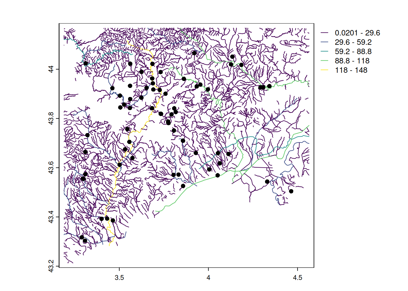
Warning
If you want to overlay multiple spatial object with base plot from sf, don’t forget to use the argument reset=FALSE in the first plot().
plot(river_sf["length_km"], reset = FALSE, axes = TRUE)
plot(pt_otter, add = TRUE)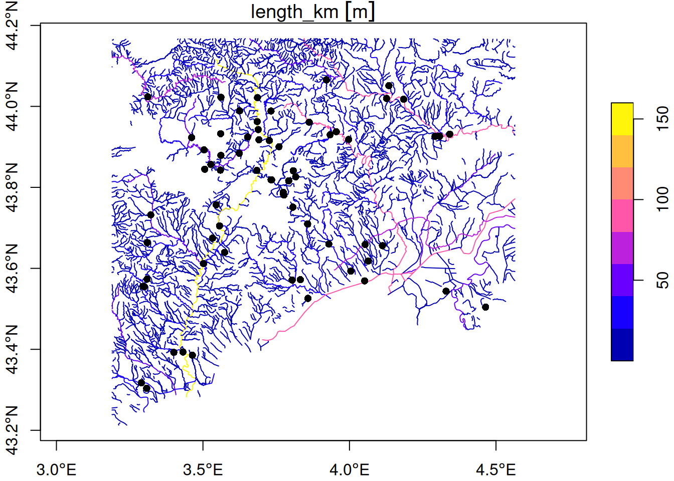
Calculate distance to the nearest line
TipThe ecologist mind
At which distance from a river were the otters observed?
To calculate distance among objects, we use the function terra::distance().
Before comparing two spatial objects, it is recommended to plot them (as in the previous figure) and make sure their projection systems are the same and the extents match. Do not use the package mapview because it will automatically project the datasets.
# make sure the spatial objects have the same projection
crs(river) == crs(pt_otter)[1] TRUE# calculate the distance between all points and lines
distance_matrix <- distance(pt_otter, river)
# get which river is the closest
nearest_river <- apply(distance_matrix, 1, which.min)
# get the nearest distance
nearest_distance <- apply(distance_matrix, 1, min)
Warning
Be aware that the newly added function terra::nearest() is not as precise as the approach shown above (as in terra 1.8-70, 03/11/2025).
In sf, the same procedure as in terra can be followed with sf::st_distance(). However it is much faster to use a two-step process: (1) find the closest river with sf::st_nearest_feature() and (2) calculate the distance between points and their closest river with sf::st_distance().
# Step 1: Find index of nearest line for each point
nearest_river_sf <- st_nearest_feature(st_as_sf(pt_otter), river_sf)The object nearest_river_sf is a vector containing the index of the closest river for each observation.
# Step 2: Calculate distance only to the nearest line
nearest_distance_sf <- st_distance(
st_as_sf(pt_otter),
river_sf[nearest_river_sf, ],
by_element = TRUE
)boxplot(nearest_distance, ylab = "distance to river (m)")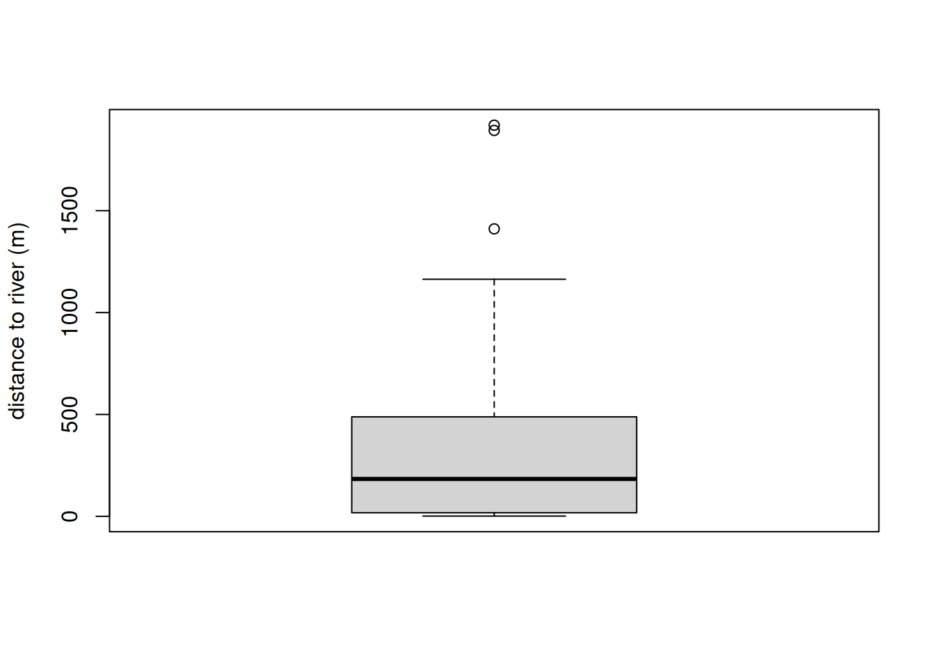
NoteYour turn
- Which are the rivers with most sights of otters?
- Make a map with the distance to river and visually check the coherence of the calculation.
- (Reflexion) What can be the factors explaining the few outliers with large distances (>1km)?
Click to see the answer 1
table(river$toponyme[nearest_river]) |>
sort(decreasing = TRUE) |>
head(5)
l'Hérault
8
la Vis
8
le Lamalou
4
Canal d'Irrigation du Bas Rhône-Languedoc ou Canal Philippe Lamour
3
Canal de Peccais à Sylvéréal
3 Click to see the answer 2
# add the distance to river to the spatial object
pt_otter$dist_river <- nearest_distance
# make an interactive map which is best to check the calculation
mapview(river) +
mapview(pt_otter, z = "dist_river")