Grid

Summary

This tutorial explores how to create a regular grid and transform spatial informations into a grid with terra package:

project spatial data to a commun CRS with terra::project()
transform vectors to raster with terra::rasterize()
match different raster grids with terra::resample()

The ecologist mind

For modeling, it is often needed to get all spatial data into a commun grid. For instance, among the spatial informations that we have seen in the previous chapter, which factors explain best the number of observations of otters?

Setup

Follow the setup instructions if you haven’t followed previous tutorials

If haven’t done it already, please follow the setup instructions.

Let’s start with loading the required packages.

suppressPackageStartupMessages({
  library(mapview)
  library(here)
  library(terra)
})

Now load all the datasets attached to the observations of otters recorded in 2021 within a 50km buffer from Montpellier, France.

pt_otter <- vect(here("data", "gbif_otter_2021_mpl50km.gpkg"))
river <- vect(here("data", "BDCARTO-River_mpl50km.gpkg"))
landuse <- vect(here("data", "BDCARTO-LULC_mpl50km.shp"))
bdalti <- rast(here("data", "BDALTI_mpl50km.tif"))
temperature <- rast(here("data", "CHELSA_monthly_tas_2015_2021.tif"))

Create a grid

Creating a grid requires a defined spatial resolution and a projection system. These choices depend on your dataset, its extent, and your modeling objectives.

In our case, we will create a grid of 5km around the otters observations using the Lambert-93 projection (EPSG:2154).

The function terra::rast() can create empty grid from the extent of a given spatial object. Here we provide the otters observation (projected in EPSG 2154) as the extent of our grid.

pt_2154 <- project(pt_otter, "EPSG:2154")
res <- 5000 # 5km grid
grid <- rast(pt_2154, res = res)
grid

class       : SpatRaster 
size        : 17, 19, 1  (nrow, ncol, nlyr)
resolution  : 5000, 5000  (x, y)
extent      : 723524.6, 818524.6, 6245001, 6330001  (xmin, xmax, ymin, ymax)
coord. ref. : RGF93 v1 / Lambert-93 (EPSG:2154)

Points to grid

The function terra::rasterize() transform vectors to raster. Its argument fun=count defines that the values in the cells are the number of points. The argument background=0 set that the value of the cells with no observation will be 0, instead of NA by default.

grid_nobs <- rasterize(pt_2154, grid, fun = "count", background = 0)

plot(grid_nobs, main = "Number of otter observations")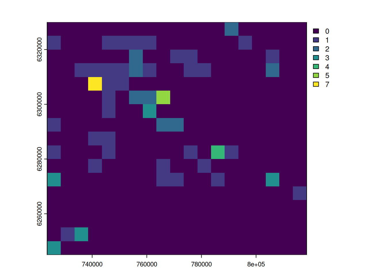

Lines to grid

To calculate the length of rivers within a grid cell, we use the function terra::rasterizeGeom(). Its argument fun=length defines that the values in the cells are the length of the rivers.

river_2154 <- project(river, "EPSG:2154")

grid_river <- rasterizeGeom(river_2154, grid, fun = "length")
plot(grid_river, main = "Length of rivers", plg = list(title = "(m)"))

Polygon to grid

To calculate the percentage of forest in the grid cells, we need first to consider only forest polygons. Then the function terra::rasterize() with the option cover=TRUE calculates the percentage of forest cover per grid cell.

# select only the forest
forest <- landuse[landuse$nature == "Forêt"]
# project the polygons
forest_2154 <- project(forest, "EPSG:2154")
# rasterize
grid_forest <- rasterize(forest_2154, grid, cover = TRUE, background = 0)

plot(grid_forest, main = "Forest cover", plg = list(title = "(%)"))

Resample raster

For rasters, we need to transform the original grid to the desired resolution and extent. This operation is done with the function terra::resample(). Be careful, this operation degrades the quality of the original raster. Each cell get the weighted average of the neighboring cells.

Elevation

grid_alti <- resample(bdalti, grid, method = "bilinear")
plot(grid_alti, main = "Elevation", plg = list(title = "(m)"))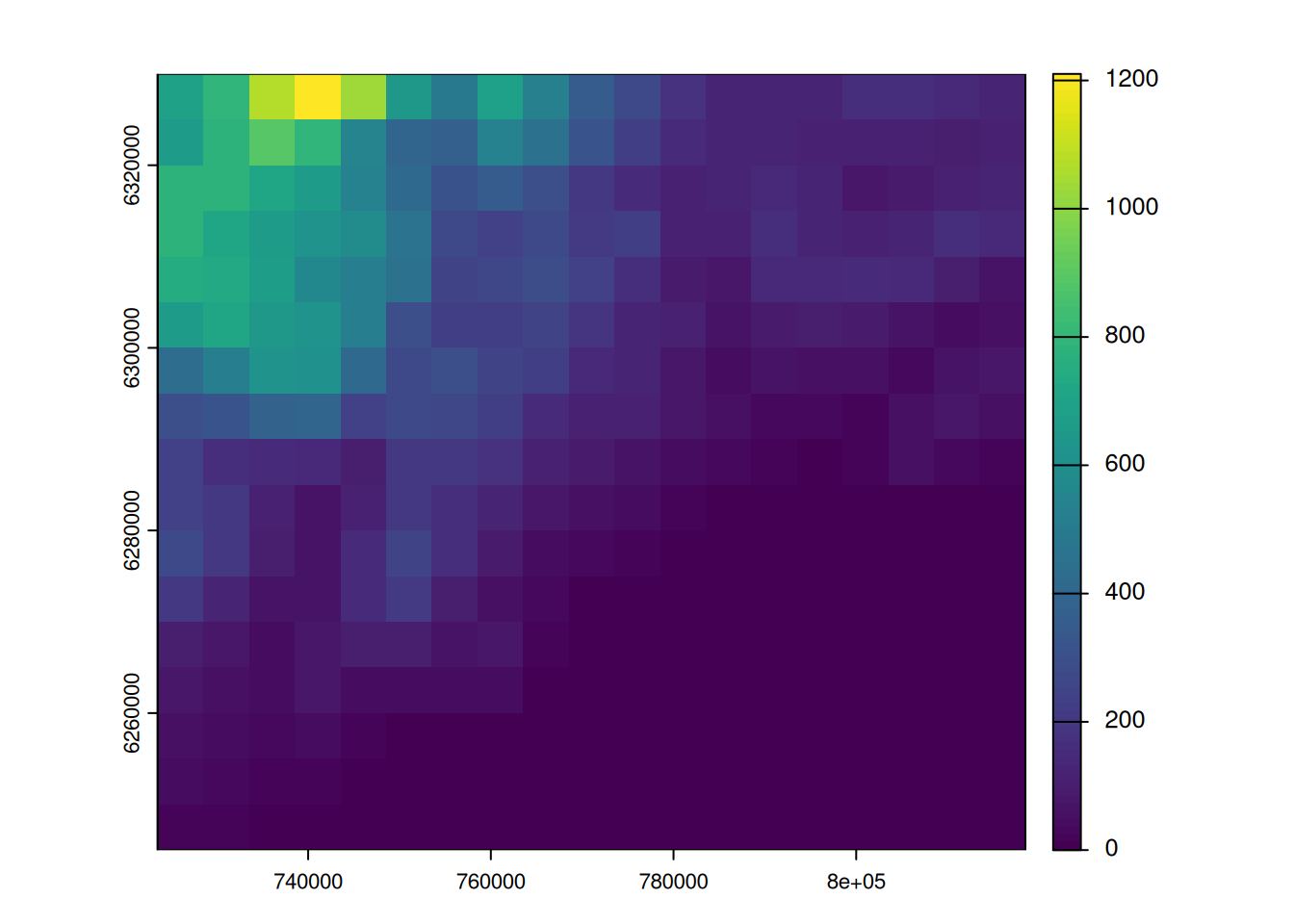

Temperature

For CHELSA temperature rasters, we will keep only a summary of 2021: the average temperature over the 12 months of 2021. So we will (1) select only layers that correspond to 2021 (year of the observations) (2) calculate the average, (3) project the raster, and (4) resample to the desired grid.

#1 select the layers corresponding to 2021
in_2021 <- grep("2021", names(temperature))
monthly_temp <- subset(temperature, in_2021)
#2. calculate the average temperature in 2021
annual_temp <- mean(monthly_temp, na.rm = TRUE)
# 3. project to EPSG 2154
temp_2154 <- project(annual_temp, "EPSG:2154")
# 4. resample to grid
grid_temp <- resample(temp_2154, grid, "bilinear")

plot(grid_temp, main = "Av. temperature", plg = list(title = "(K)"))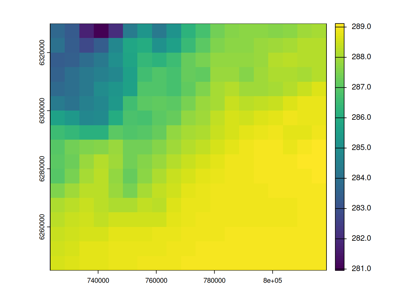

Merge all together

In terra, we can group SpatRaster objects into a single one if they all share the same grid. We will then get one grid and multiple layers (also called band) with the different informations.

# merge all information into one single output
out <- c(grid_nobs, grid_river, grid_forest, grid_alti, grid_temp)
# we rename the layers to keep information of units
names(out) <- c("nobs", "river_m", "forest", "elevation_m", "temperature_K")

out

class       : SpatRaster 
size        : 17, 19, 5  (nrow, ncol, nlyr)
resolution  : 5000, 5000  (x, y)
extent      : 723524.6, 818524.6, 6245001, 6330001  (xmin, xmax, ymin, ymax)
coord. ref. : RGF93 v1 / Lambert-93 (EPSG:2154) 
source(s)   : memory
names       : nobs,  river_m,    forest, elevation_m, temperature_K 
min values  :    0,     0.00, 0.0000000,       0.000,      280.9530 
max values  :    7, 56861.96, 0.9665119,    1210.254,      289.1167

plot(out)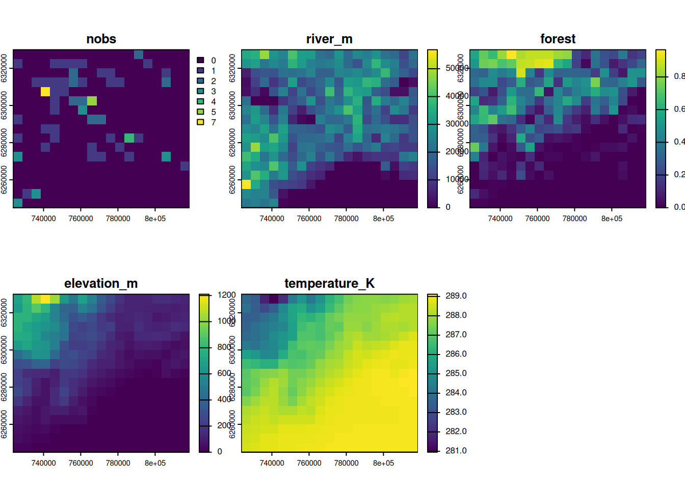

Your turn

Our grid includes the Mediterranean Sea, but the otter observations were only made on land. Mask the created raster with the land boundary of France (as in the Chapter Rasters).

Click to see the answer

# get the border of the country (level = 0)
france_border <- readRDS(here("data", "gadm41_FRA_0_pk.rds"))
# or directly from geodata
# france_border <- geodata::gadm("FRA", level = 0, path = here("data"))
# project the coast in Lambert-93
france_2154 <- project(france_border, crs(bdalti))
# mask (=set to NA) the pixels that are not in the polygon
out_masked <- mask(out, france_2154)
plot(out_masked)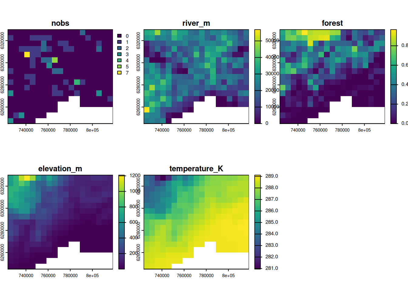

Simple linear model

The dataset is made of observations gathered without proper sampling schemes, and with potentially many biases. For such data (opportunistic presence-only data), it is recommended to use species occupancy models.

Yet, for our little case study we will do a simple linear model.

# transform the spatial raster data as data.frame
df <- data.frame(out_masked)

# make a simple linear model
m1 <- lm(nobs ~ river_m + forest + elevation_m + temperature_K, data = df)
summary(m1)


Call:
lm(formula = nobs ~ river_m + forest + elevation_m + temperature_K, 
    data = df)

Residuals:
    Min      1Q  Median      3Q     Max 
-0.6221 -0.3503 -0.2522 -0.0324  6.5679 

Coefficients:
                Estimate Std. Error t value Pr(>|t|)   
(Intercept)    2.584e+02  8.709e+01   2.967  0.00327 **
river_m       -6.591e-08  4.862e-06  -0.014  0.98920   
forest        -2.689e-01  2.718e-01  -0.989  0.32331   
elevation_m   -5.833e-03  2.081e-03  -2.803  0.00543 **
temperature_K -8.936e-01  3.014e-01  -2.965  0.00329 **
---
Signif. codes:  0 '***' 0.001 '**' 0.01 '*' 0.05 '.' 0.1 ' ' 1

Residual standard error: 0.7884 on 276 degrees of freedom
Multiple R-squared:  0.03659,   Adjusted R-squared:  0.02262 
F-statistic:  2.62 on 4 and 276 DF,  p-value: 0.03531

The linear model is definitely not a good fit to our data (R2 is only 0.03). Moreover, there is strong collinearity between elevation and temperature, and the residuals are not normally distributed (to see how wrong is our model, try plot(m1)).
It might help if we use generalized mixed models. For zero-inflated datasets, one option is to make two separate models: (1) model the presence-absence as a binomial variable, and (2) model the number of observations with poisson distribution. Yet, in our case the main issue here is the high number of ‘false’ zeros (opportunistic observations, presence-only information) which can only be resolved with species occupancy models (e.g. spOccupancy).

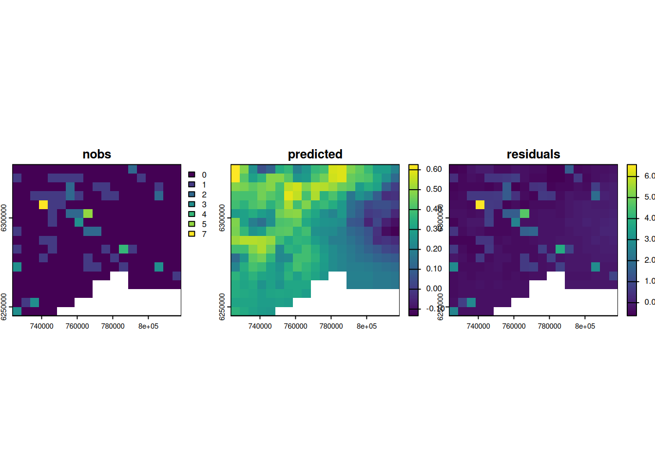
However, it is always recommended to spatially visualize the predictions and the residuals.

# set new empty grids
out_masked$predicted <- rast(grid)
out_masked$residuals <- rast(grid)
# add values of prediction and residuals where there is no NA
out_masked$predicted[!is.na(out_masked$nobs)] <- predict(m1)
out_masked$residuals[!is.na(out_masked$nobs)] <- residuals(m1)
# show and compare the observation, prediction and residuals
plot(out_masked, c("nobs", "predicted", "residuals"), nc = 3)