Polygons

Summary

This tutorial explores how to handle spatial polygons in R with terra package:

read a spatial object with terra::vect()
calculate the area of polygons with terra::expanse()
extract values of polygons to points with terra::extract()
create buffers around points with terra::buffer()
find intersection among two polygon layers with terra::intersect()

The ecologist mind

In which type of habitats were the otters observed? To answer this question, we will need to discover another type of spatial vector: polygons.

Setup

Follow the setup instructions if you haven’t followed the tutorial on points

If haven’t done it already, please follow the setup instructions. Let’s start with loading the required packages.

suppressPackageStartupMessages({
  library(mapview)
  library(here)
  library(sf)
  library(terra)
})

pt_otter <- vect(here("data", "gbif_otter_2021_mpl50km.gpkg"))

pt_otter <- vect(
  "https://github.com/FRBCesab/spatial-r/raw/main/data/gbif_otter_2021_mpl50km.gpkg"
)

Load polygons from a shapefile

In this example, we will load land cover information for the area of interest from IGN data BD CARTO.

Note that this dataset has rough resolution (OSO or Corine land cover would be more suited for real analysis), but it’s perfect for our illustration and learning purposes.

You can load vector data with the function terra::vect().

landuse <- vect(here("data", "BDCARTO-LULC_mpl50km.shp"))

landuse_sf <- st_read(here("data", "BDCARTO-LULC_mpl50km.shp"))

Reading layer `BDCARTO-LULC_mpl50km' from data source 
  `/home/romain/GitHub/spatial-r/data/BDCARTO-LULC_mpl50km.shp' 
  using driver `ESRI Shapefile'
Simple feature collection with 2910 features and 3 fields
Geometry type: MULTIPOLYGON
Dimension:     XY
Bounding box:  xmin: 3.18983 ymin: 43.20373 xmax: 4.56447 ymax: 44.16754
Geodetic CRS:  WGS 84

If you don’t have the data locally (and won’t use it repeatedly), you can load it directly with:

landuse <- vect(
  "https://github.com/FRBCesab/spatial-r/raw/refs/heads/main/data/BDCARTO-LULC_mpl50km.shp"
)

Your turn

How many different polygons are used in the land cover of our study area?
What is the coordinate reference system (CRS) of the loaded river data?
How many land cover classes are there? Which class has the most polygons?

Click to see the answer

There was 2910 polygons in the dataset. You can access it with dim(landuse), nrow(landuse) or just by typing landuse in the console.
The coordinates are in WGS 84 (EPSG 4326). You can access this information with crs(landuse, describe = TRUE) (or in sf with st_crs(landuse_sf)).
The column that stored the cover classes is nature. You could identify it with head(landuse) or names(landuse). There are 12 land cover classes, Prairie is the class with most polygons (table(landuse$nature)).

Visualization

Before comparing two spatial objects (the otters observations and the land cover), it is recommended to plot them and make sure their projection systems are the same and the extents match.
Do not use the package mapview because it will automatically project the datasets.

plot(landuse, y = "nature", border = NA)
plot(pt_otter, add = TRUE)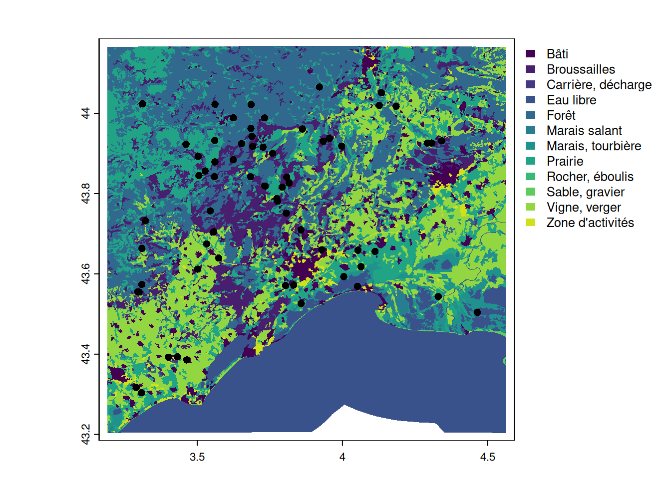

plot(landuse_sf["nature"], reset = FALSE, border = FALSE, axes = TRUE)
plot(pt_otter, add = TRUE, pch = 16)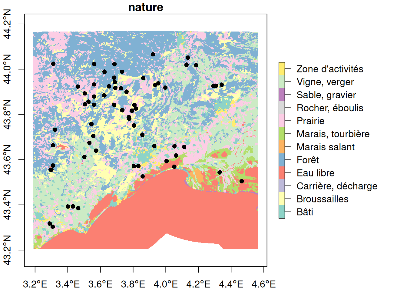

Warning

When you want to overlay multiple spatial object with base plot from sf, don’t forget to use the argument reset=FALSE.

Calculate area

The ecologist mind

What is the dominant land cover in our study area?

The function terra::expanse() calculates the area in $m^2$. When calculating areas, be careful with projection systems. Some are not suited to calculate areas. Prefer equal-area projections or use local projection systems (if your study area is small).

Luckily, the package terra calculates by default the geodesic area (based on lat/long coordinates and considering Earth’s curvature) which is the most accurate estimate and avoid errors due to wrongly used projection system.

# calculate the area in ha
area_polygons <- expanse(landuse) * 0.0001
# store the area as atribute
landuse$area_ha <- as.numeric(area_polygons)

In sf, it is recommended to project the dataset to a equal area projection, such as the Lambert azimuthal equal-area for Europe EPSG:3035.

# project land cover to an equal-area projection system
landuse_3035 <- st_transform(landuse_sf, crs = 3035)
# calculate area of polygons (in hectare)
area_polygons <- st_area(landuse_3035) * 0.0001
# store as attribute in landuse
landuse_3035$area_ha <- as.numeric(area_polygons)

Your turn

Which are the largest land cover classes in our study area? Why?

Click to see the answer

# see area per land use classes
area_landuse <- tapply(landuse$area_ha, landuse$nature, sum)
sort(area_landuse)

   Rocher, éboulis Carrière, décharge     Sable, gravier      Marais salant 
          37.78454         1916.22618         2353.14638         3455.79520 
  Zone d'activités  Marais, tourbière               Bâti       Broussailles 
       15224.16350        29467.47117        55654.39730        97923.34835 
     Vigne, verger            Prairie          Eau libre              Forêt 
      206514.68518       206833.73332       272561.76875       278134.18692

The categories Forêt (=forest) and Eau libre (=running water) are the largest land covers. As it can be seen in the previous map, large part of the Mediterranean Sea is included in the land cover data.

Mask the sea

The ecologist mind

Our study area was defined as a square buffer around Montpellier. This area include the Mediterranean Sea. It is recommended to mask the sea in order to consider only areas where otters could have been potentially spotted.

There are two approaches to mask an area: (1) identify which area to remove from the data itself, or (2) use a mask from another data source (this approach will be shown when dealing with rasters). In this case, it is easier and more accurate to detect directly from the data which polygons to remove. In fact, the largest polygon corresponds to the Mediterranean Sea. So we just need to remove it.

# the largest polygon correspond to the mediterranean
landuse$nature[which.max(landuse$area_ha)]

[1] "Eau libre"

# remove the largest polygon
landuse_nomed <- landuse[-which.max(landuse$area_ha), ]
# visually verify the output
plot(landuse_nomed, y = "nature", border = NA)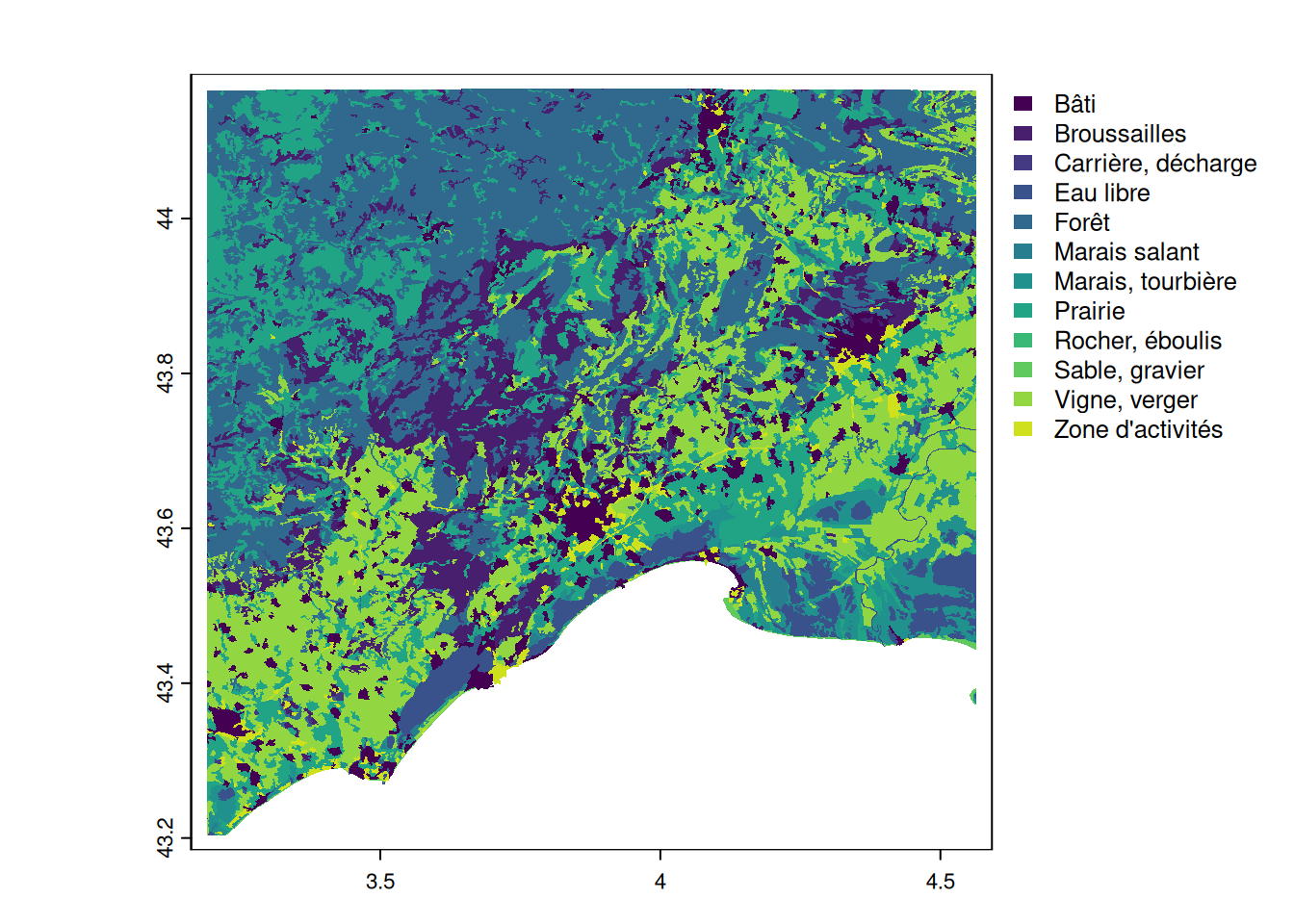

Then we can recalculate the percentage of land cover per class.

cover_ha <- tapply(landuse_nomed$area_ha, landuse_nomed$nature, sum)
# percentage of land cover classes in the terrestrial study area
cover_perc <- cover_ha / sum(cover_ha) * 100
#show rounded values
round(cover_perc, 2)

              Bâti       Broussailles Carrière, décharge          Eau libre 
              5.98              10.52               0.21               3.61 
             Forêt      Marais salant  Marais, tourbière            Prairie 
             29.87               0.37               3.16              22.21 
   Rocher, éboulis     Sable, gravier      Vigne, verger   Zone d'activités 
              0.00               0.25              22.18               1.64

Polygons to points

The ecologist mind

What is the land cover class at the location of the otters observations?

We can extract the land cover class of the points with terra::extract():

pt_landcover <- extract(landuse, pt_otter)

We can extract the land cover class of the points with sf::st_join():

pt_landcover <- st_join(st_as_sf(pt_otter), landuse_sf)

# see the number of observations per land use classes
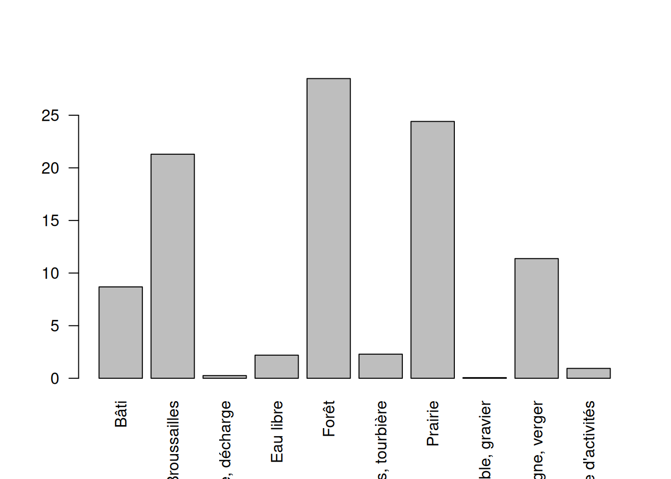
table(pt_landcover$nature)


             Bâti      Broussailles         Eau libre             Forêt 
                8                17                 1                29 
Marais, tourbière           Prairie     Vigne, verger 
                3                16                 9

Your turn

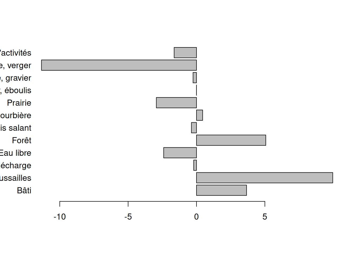
[stat] Which classes are over- or under- represented compare to the distribution of classes over the whole study area?

Click to see the answer

# calculate the percentage of otters observations per class
cover_obs_perc <- table(pt_landcover$nature) / nrow(pt_landcover) * 100
# match all classes with the one from the observations
m0 <- match(names(cover_perc), names(cover_obs_perc))
# create a data.frame
cover <- data.frame(
  class = names(cover_perc),
  all = as.numeric(cover_perc),
  obs = as.numeric(cover_obs_perc[m0])
)
# non matchin elements = 0%
cover[is.na(cover)] <- 0
# calculate the difference between observed and expected
cover$delta <- cover$obs - cover$all
# add left margin to the plot
par(mar = c(4, 8, 4, 1))
barplot(
  cover$delta,
  horiz = TRUE,
  names = cover$class,
  las = 1,
  xlab = "Difference between observed and expected cover (%)"
)

Polygons to polygons

The ecologist mind

What is the land cover distribution around the locations of the otters observations?

To characterize the area surrounding the observations, we need to (!) create buffers, (2) calculate the intersection among the buffers and the land cover, and (3) calculate the area of the land cover classes intersecting the buffers.

Create buffer

We can create buffer with terra::buffer(). In our example, we will create buffers of 1km.

dist_buffer <- 1000 # buffer of 1000 m
poly_otter <- buffer(pt_otter, dist_buffer)

Warning

sf uses s2 when the coordinates are geographic (e.g. EPSG:4326) which creates buffers with low quality (in sf 1.0-21, tested on 03/11/2025).
It is recommended to use projected coordinates when using the function sf::st_buffer().

dist_buffer <- 1000 # buffer of 1000 m
# transform to an equal-area projection system: better for area
pt_otter_3035 <- st_as_sf(pt_otter) |> st_transform(3035)
poly_otter_3035 <- st_buffer(pt_otter_3035, dist_buffer)

Visualize buffer

For illustration, we only show the buffer around the first observation.

The parameter ext limit the map to the extent of the given spatial object.

# plot the land cover limited to the extent of the buffer
plot(landuse, y = "nature", ext = poly_otter[1])
# add the buffer as a line of width 2
plot(poly_otter[1], lwd = 2, add = TRUE)
# add the observation as a red dot
plot(pt_otter[1], col = "red", add = TRU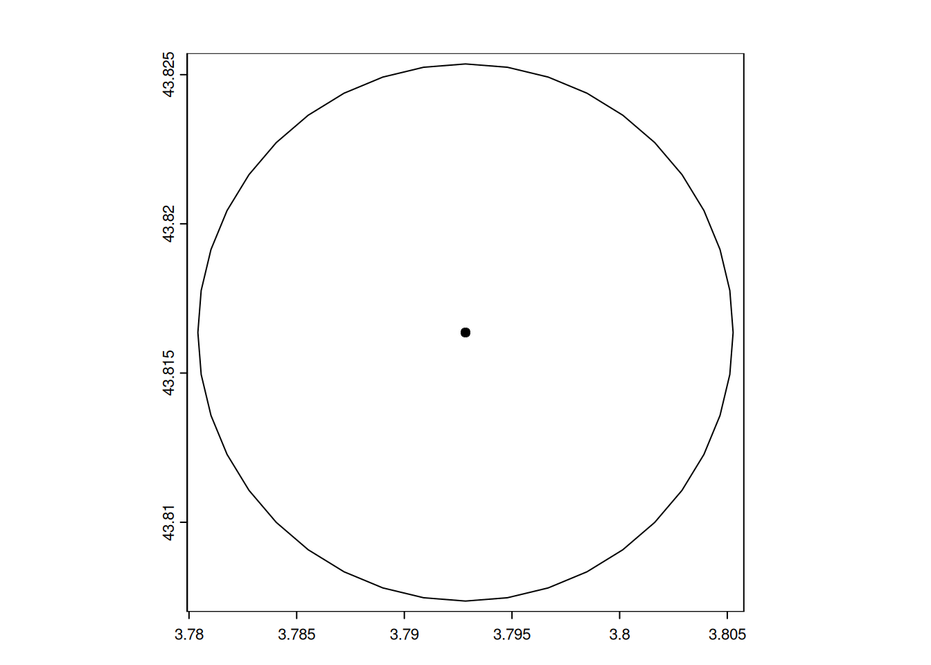E)

Your turn

What are the areas of the newly created buffers?

Click to see the answer

# calculate the area of the buffers
buffer_area <- expanse(poly_otter)
# see the distribution of the buffer areas
summary(buffer_area)

   Min. 1st Qu.  Median    Mean 3rd Qu.    Max. 
3128689 3128689 3128689 3128689 3128689 3128689

# distribution of the buffer areas from sf
summary(st_area(poly_otter_3035))

   Min. 1st Qu.  Median    Mean 3rd Qu.    Max. 
3140157 3140157 3140157 3140157 3140157 3140157

The difference with expected value of $3141593$ is due to the way buffers are defined (by default, in 40 points in terra and 120 points in sf). If you want more precise buffers, you can change the parameter quadsegs from the terra::buffer() function. The roundness of the buffers is not important for most cases. It is much more important that all buffers have the same area.

Intersection among polygons

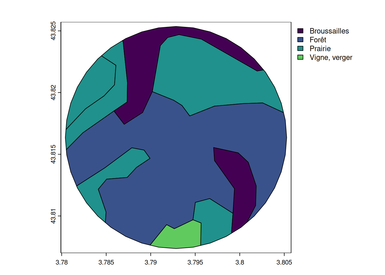
We can now intersect the buffers with the land cover information with the function terra::intersect().

buffer_landcover <- intersect(landuse, poly_otter)

# visualize the intersection
# not plotted here to lighten the webpage
# mapview(buffer_landcover, z = "nature")

# show a zoom on the land cover of the first buffer
plot(
  buffer_landcover[buffer_landcover$key %in% poly_otter$key[1]],
  y = "nature"
)

buffer_landcover_sf <- st_intersection(poly_otter_3035, landuse_3035)

Warning: attribute variables are assumed to be spatially constant throughout
all geometries

# visualize the intersection (not plotted to lighten the webpage)
# mapview(buffer_landcover, z = "nature")

Land cover area per buffer

We need to update the area of the land cover intersecting the buffers.

# Calculate area for each polygon
buffer_landcover$area_ha <- expanse(buffer_landcover) * 0.0001

# Calculate area per buffer and nature class
class_area <- tapply(
  buffer_landcover$area_ha,
  list(buffer_landcover$key, buffer_landcover$nature),
  sum
)
#replace NA by 0
class_area[is.na(class_area)] <- 0
# calculate the area of the buffer
sum_area <- rowSums(class_area)
# calculate the percentage per class
perc_class <- class_area / sum_area * 100

# add margin at the bottom
par(mar = c(7, 4, 1, 1))
barplot(apply(perc_class, 2, mean), las = 2, ylab = "Percentage land cover")