Rasters

Summary

This tutorial explores how to handle rasters in with terra package:

import a raster file with terra::rast()
mask non relevant areas with terra::mask()
extract information from rasters on points or polygons with terra::extract()

The ecologist mind

Elevation is a key geographical variable that strongly define habitats. At which elevation were the otters observed? To answer this question, we will need to discover another type of spatial data: rasters.

Setup

Follow the setup instructions if you haven’t followed the previous tutorials

If haven’t done it already, please follow the setup instructions.

Let’s start with loading the required packages.

suppressPackageStartupMessages({
  library(mapview)
  library(here)
  library(terra)
})

Load the observations of otters recorded in 2021 within a 50km buffer from Montpellier, France.

pt_otter <- vect(here("data", "gbif_otter_2021_mpl50km.gpkg"))

url_github <- "https://github.com/FRBCesab/spatial-r/raw/main/data/"
pt_otter <- vect(paste0(url_github, "gbif_otter_2021_mpl50km.gpkg"))

Load raster from a geotiff file

We will use the elevation data from IGN data BD ALTI which was aggregated at 250m resolution (instead of its original resolution of 25m). Note that the rough resolution of this dataset is perfect for our learning purpose. Yet for real analyses, you might consider finer spatial data. The function to read raster file is terra::rast()

bdalti <- rast(here("data", "BDALTI_mpl50km.tif"))

If you don’t have the data locally (and won’t use it repeatedly), you can load it directly with:

bdalti <- rast(
  "https://github.com/FRBCesab/spatial-r/raw/refs/heads/main/data/BDALTI_mpl50km.tif"
)

Rasters characteristics

bdalti

class       : SpatRaster 
size        : 432, 439, 1  (nrow, ncol, nlyr)
resolution  : 250, 250  (x, y)
extent      : 715438.3, 825188.3, 6233959, 6341959  (xmin, xmax, ymin, ymax)
coord. ref. : RGF93 v1 / Lambert-93 (EPSG:2154) 
source      : BDALTI_mpl50km.tif 
name        : BDALTI_mpl50km

The loaded raster is projected in RGF93 v1 / Lambert-93 (EPSG 2154). It is a matrix with 432 rows, 439 columns, and a spatial resolution of 250m (on x and y). All the information about terra::SpatRaster can be accessed individually. Use terra::crs() for information on the projection system, terra::ext() for the geographical extent, terra::res() for the resolution, and dim() for the dimensions (number of rows, number of columns and number of layers).

# get the name of the layer
names(bdalti)

[1] "BDALTI_mpl50km"

# rename the layer (for simplicity)
names(bdalti) <- "elevation"

We can access all values of the raster with the function terra::values(). This operation is often not needed and not recommended if you have large rasters. But it is the only way to get the distribution of all values.

# get all the values : values()
# use only for small raster
# else it takes large amount of time and memory
boxplot(values(bdalti), ylab = "elevation (m)")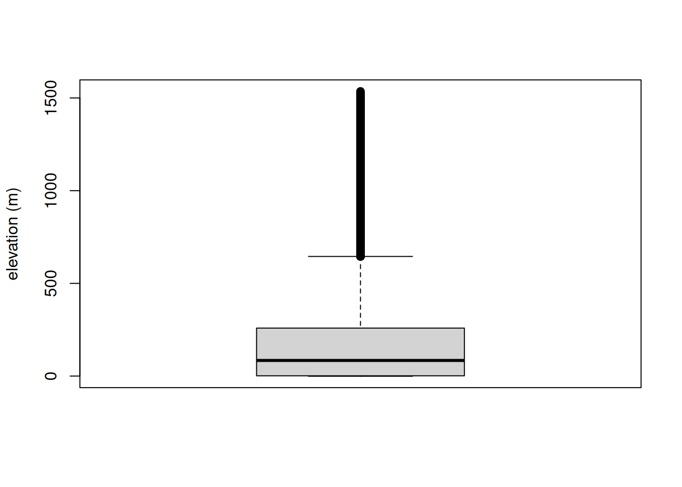

# mean elevation in our study area
summary(values(bdalti))

   elevation        
 Min.   :  -0.9723  
 1st Qu.:   1.4320  
 Median :  84.2625  
 Mean   : 198.9497  
 3rd Qu.: 258.9347  
 Max.   :1536.2190

Visualization

Similar to vectors, rasters can be visualized as static map with the function plot() or interactively with the package mapview.

plot(bdalti)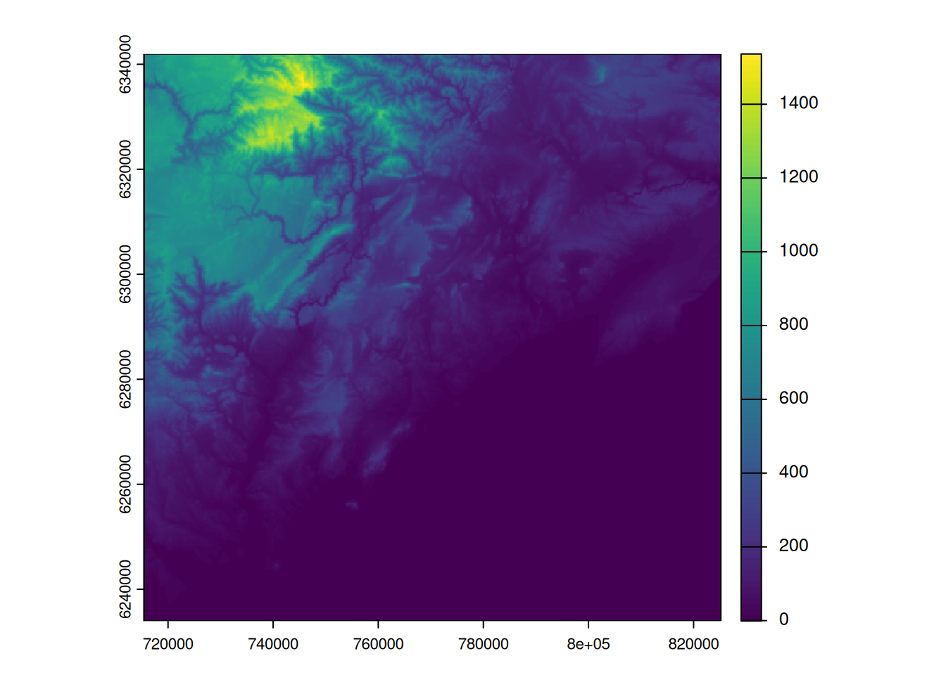

mapview(bdalti)

Mask the sea

The ecologist mind

Our study area was defined as a square buffer around Montpellier. This area include the Mediterranean Sea. It is recommended to mask the sea in order to consider only areas where otters could have been potentially spotted.

To mask all pixels that don’t fit our study area (the terrestrial environment 50km around Montpellier), we need (1) to get the borders of France from GADM, (2) project the border to match the elevation raster, and (3) mask the area that are not in the country polygon with the function terra::mask().

# get the border of the country
france_border <- readRDS(here("data", "gadm41_FRA_0_pk.rds"))

# get the border of the country (level = 0)
france_border <- geodata::gadm("FRA", level = 0, path = here("data"))

# project the coast in Lambert-93
france_2154 <- project(france_border, crs(bdalti))

# mask (=set to NA) the pixels that are not in the polygon
alti_masked <- mask(bdalti, france_2154)

# visualize the new raster without the Mediterranean Sea
plot(alti_masked)

# mean elevation in our study area (excluding sea)
summary(values(alti_masked), na.rm = TRUE)

   elevation       
 Min.   :  -0.972  
 1st Qu.:  45.448  
 Median : 138.845  
 Mean   : 252.695  
 3rd Qu.: 339.775  
 Max.   :1536.219  
 NA's   :40336

Raster to points

The ecologist mind

Now that we have loaded the elevation data, let’s get the elevation at the location of otters observations.

Checking projections and extent

Remember that before comparing two spatial objects, it is always a good idea to map them together.

plot(alti_masked)
plot(pt_otter, add = TRUE)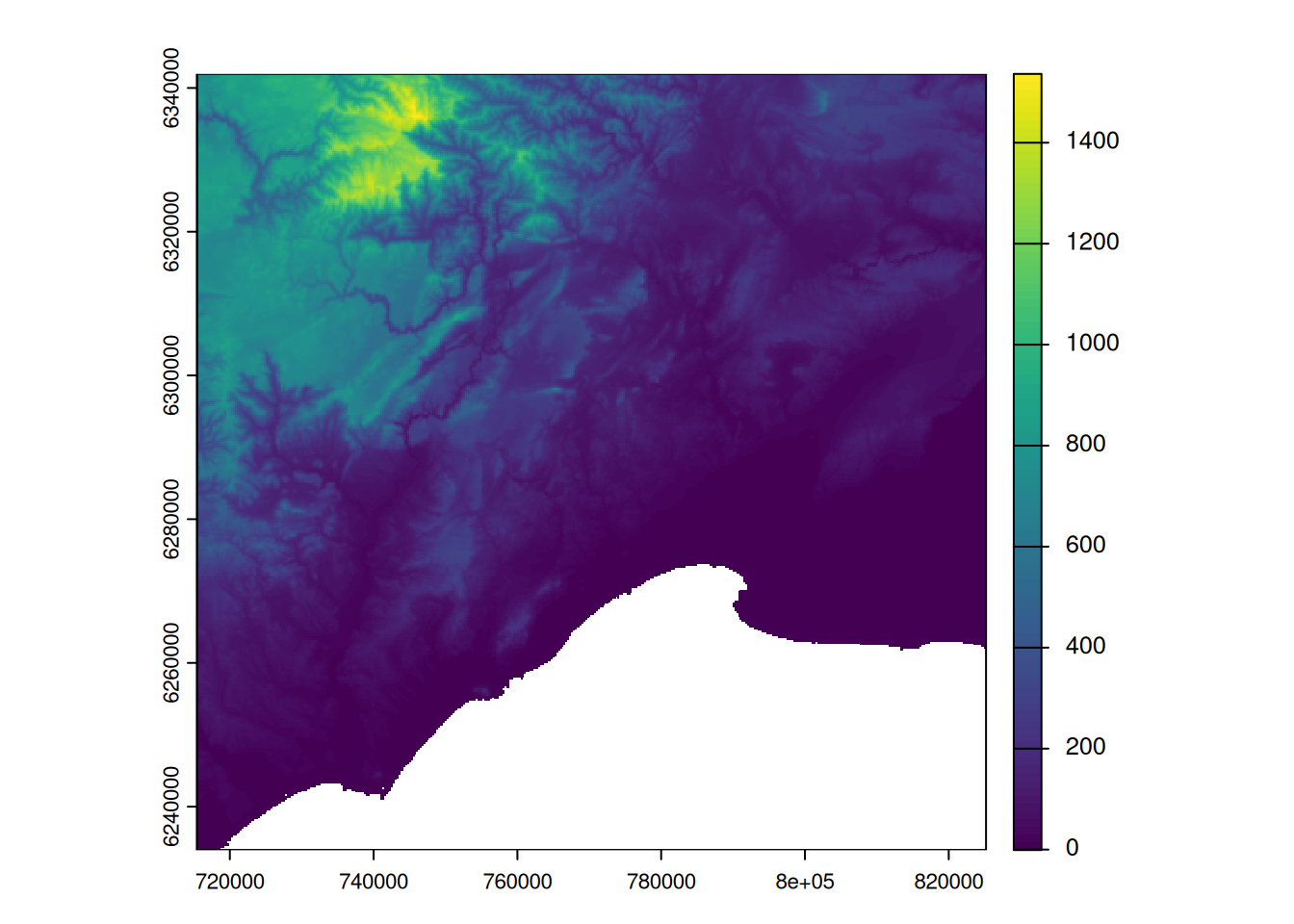

Your turn

Why can’t you see the otters observations? How to fix this problem?

Click to see the answer

Indeed, the spatial points with the otters observations don’t share the same projection than the elevation raster. We need to project the spatial points to the CRS of the elevation data.

Important

It is not recommended to project raster objects. When you have the choice, it is always better to project vector data to the CRS of the raster.

# the projection systems are not matching
crs(bdalti) == crs(pt_otter)

[1] FALSE

# let's project the otter observations to the raster's CRS
pt_2154 <- project(pt_otter, crs(bdalti))

# now we can check that the points overlay the elevation data
plot(alti_masked)
plot(pt_2154, col = "red", add = TRUE)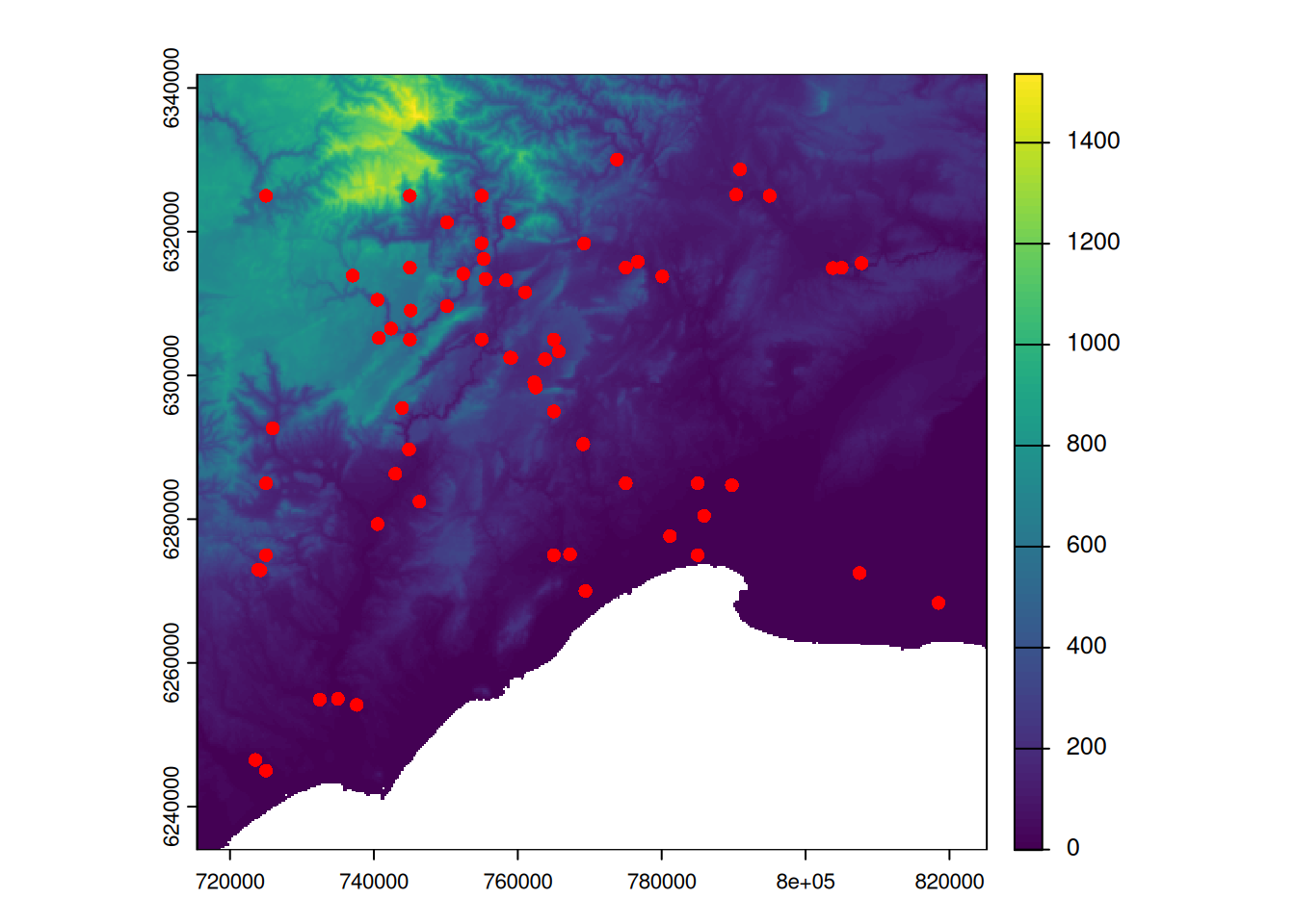

Extraction of elevation values

Now we can use the function terra::extract() to get the elevation of the observations.

pt_alti <- extract(alti_masked, pt_2154)

# visualize the extracted values
boxplot(pt_alti$elevation, ylab = "elevation (m)")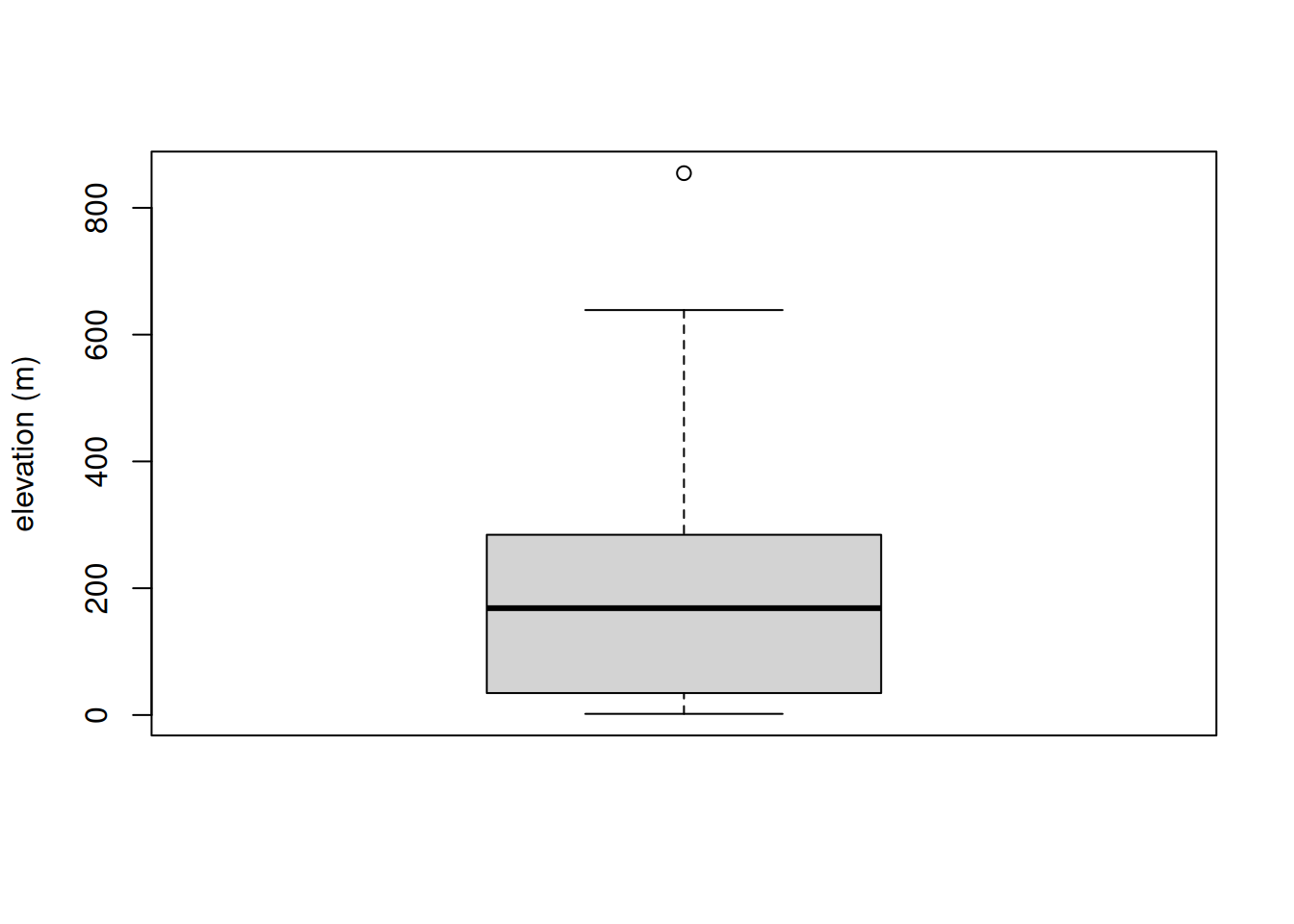

Your turn

Compare the extracted elevation with the elevation provided with GBIF (in the attribute table of the points).
Are otters changing their elevation distribution depending on the time of the year? In other words, can we see differences in elevation depending on the time of the year in which the observations were made?

Click to see the answer 1

# check with recorded
plot(
  pt_alti$elevation,
  pt_otter$elevation,
  xlab = "elevation (m) GBIF values",
  ylab = "elevation (m) BDALTI values",
  asp = 1
)
# add identity line
abline(a = 0, b = 1)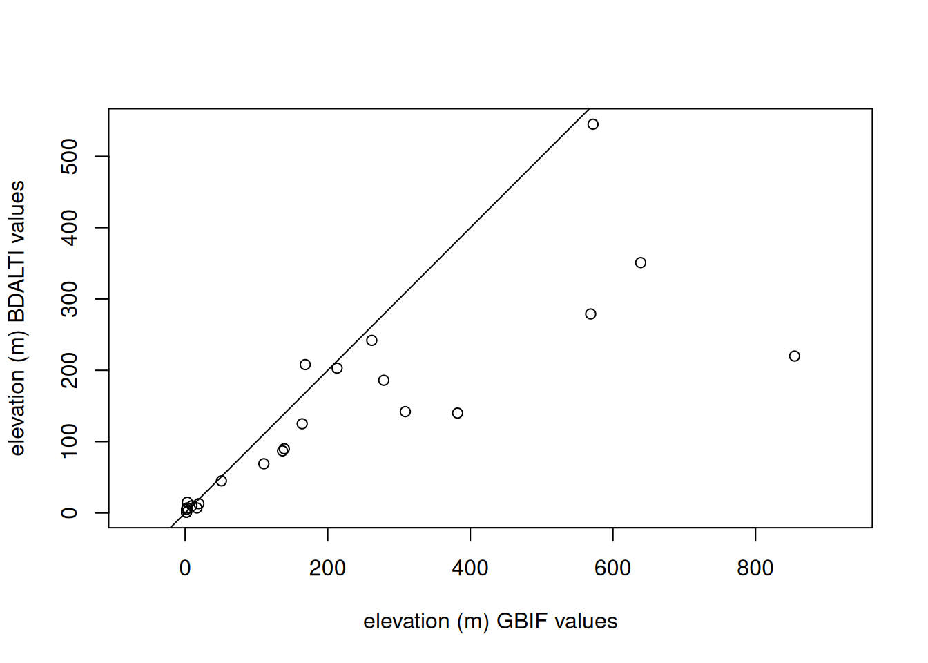

Click to see the answer 2

boxplot(
  pt_alti$elevation ~ pt_otter$month,
  xlab = "Month of observation",
  ylab = "elevation (m)"
)

Raster to polygons

The ecologist mind

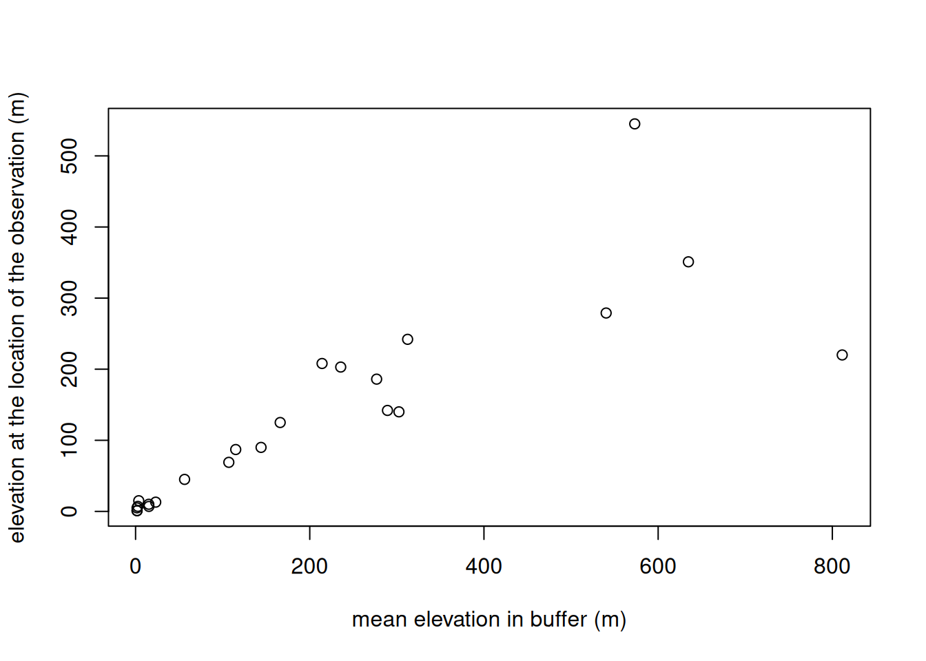
What is the elevation around the locations of the otters observations?

Create buffer

We can create buffer with terra::buffer(). It is recommended to work on geographic coordinates (latitude/longitude), or in an equal-area projection (which is not the case of Lambert-93). Hence, we will first create the buffer in lat/long and then project them in Lambert-93.

dist_buffer <- 1000 # buffer of 1000 m
poly_otter <- buffer(pt_otter, dist_buffer)
# project to Lambert-93
poly_2154 <- project(poly_otter, crs(bdalti))

Nerdy

Curious to know why it is recommended to create buffer in lat/long with terra? Try it out. Create buffer in Lambert-93 and check whether all buffers have the same size.

Click to see the answer

# create buffer directly in Lamber 93
buffer_2154 <- buffer(pt_2154, 1000)
# get the standard deviation of the area of the buffers
sd(expanse(buffer_2154))

[1] 1002.459

# and compare it with the buffers created in lat/long
sd(expanse(poly_2154))

[1] 3.117107e-05

Get average elevation

The function terra::extract() can summarize the information per polygon with the parameter fun. If no function is provided, it will extract all values that intersect the polygons.

It is recommended to use the parameter exact=TRUE to get the weighted mean based on the fraction of each cell that is covered (but computation is slower).

mean_alti <- extract(alti_masked, poly_2154, fun = mean, exact = TRUE)

plot(
  mean_alti$elevation,
  pt_otter$elevation,
  xlab = "mean elevation in buffer (m)",
  ylab = "elevation at the observation (m)"
)

Get all values within buffers

To understand how the function extract works, it is helpful to extract all values.

full_alti <- extract(alti_masked, poly_2154, exact = TRUE)
head(full_alti)

  ID elevation   fraction
1  1  232.2320 0.04703028
2  1  222.9880 0.13675144
3  1  218.9846 0.02927423
4  1  203.8373 0.06348854
5  1  231.5380 0.63766422
6  1  221.8044 0.98195943

Each row is a cell that is matching a polygon. elevation is the elevation value of the cell, fraction is the fraction of the cell covered by the polygon, and ID is the identifier of the intersecting polygon.

We can calculate the number of different pixels that intersects the polygon.

npixels <- table(full_alti$ID)
table(npixels)

npixels
63 64 65 66 67 68 69 
 1  3  2  7 18 44  8

The polygons intersect between 63 and 69 pixels, but some are partially intersecting. Let’s now calculate the surface (in number of pixels) covered by the buffer

area_per_id <- tapply(full_alti$fraction, full_alti$ID, sum)
summary(area_per_id)

   Min. 1st Qu.  Median    Mean 3rd Qu.    Max. 
  50.05   50.07   50.07   50.08   50.09   50.12

The buffers cover an area equivalent to 50 full pixels.

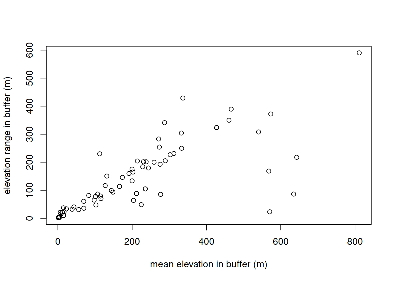
An interesting ecological variable that we can calculate with data for each pixel is the range of the elevation found within the buffer.

drange_alti <- tapply(full_alti$elevation, full_alti$ID, function(x) {
  diff(range(x))
})

plot(
  mean_alti$elevation,
  drange_alti,
  xlab = "mean elevation in buffer (m)",
  ylab = "elevation range in buffer (m)"
)