The aim of the package chessboard is to provide tools to
work with directed (asymmetric) and
undirected (symmetrical) spatial (or non-spatial)
networks. It implements different methods to detect
neighbors, all based on the chess game (it goes beyond the rook and the
queen available in many R packages) to create complex connectivity
scenarios.
chessboard aims to easily create various network
objects, including:
- node list, i.e. a list of all nodes of the network;
- edge list, i.e. a list of all edges (links) between pairs of nodes;
-
connectivity matrix, i.e. a binary matrix of
dimensions
n x n, wherenis the number of nodes (sampling units) indicating the presence (1) or the absence (0) of an edge (link) between pairs of nodes.
# Setup ----
library("chessboard")
library("ggplot2")
library("patchwork")
Network properties
chessboard can handle spatial networks, but it does not
explicitly use geographical coordinates to find neighbors (it is not
based on spatial distance). Instead, it identifies neighbors according
to node labels (i.e. the node position on a
two-dimension chessboard) and a specific method (pawn, fool, rook,
bishop, knight, queen, wizard, etc.) derived from the chess game.
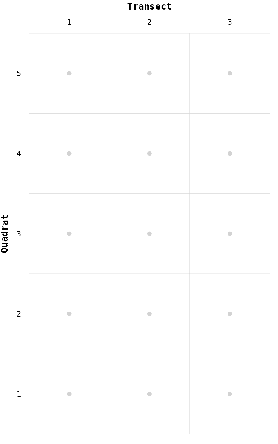
Figure 1. Network as a chessboard
The package chessboard is designed to work with
two-dimensional networks (i.e. sampling on a regular grid), where one
dimension is called transect and the other is called
quadrat. By convention, the dimension
transect corresponds to the x-axis, and the
quadrat corresponds to the y-axis (Fig. 1).
chessboard can also deal with one-dimensional network
(either transect-only or
quadrat-only).
The network can be undirected or directed. If the network is directed, it will have (by default) these two orientations:
- from bottom to top (along transect) for quadrats
- from left to right (along quadrat) for transects
Neighbors detection
chessboard implements the following rules to detect
neighbors and to create edges:
the degree of neighborhood: the number of adjacent nodes that will be used to create direct edges.
the orientation of neighborhood: can neighbors be detected horizontally, vertically and/or diagonally?
the direction of neighborhood: does the sampling has a main direction? This can be particularly relevant for directed networks (e.g. rivers).
Workflow
The Figure 2 shows the general workflow and the main features of
chessboard.
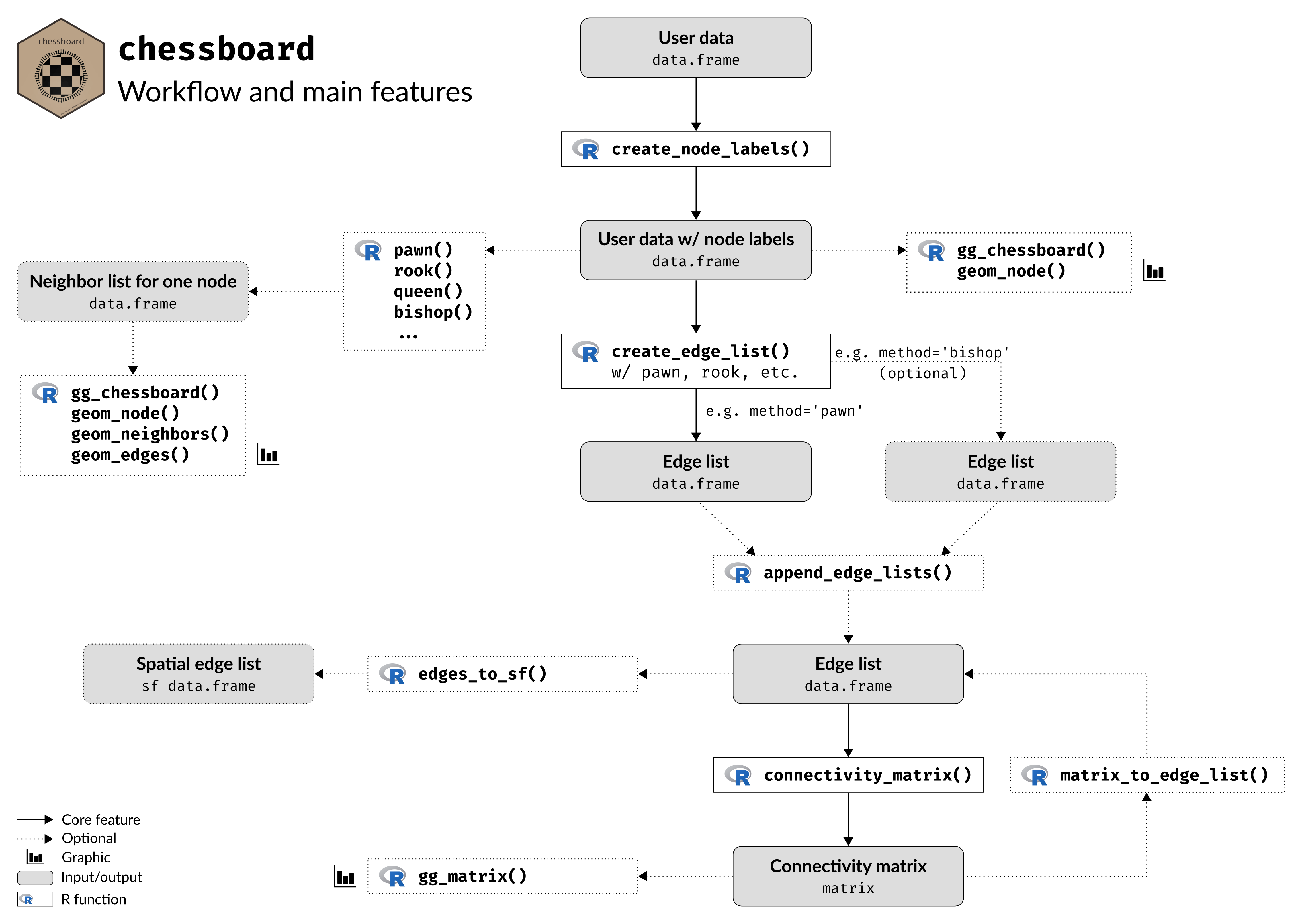
Figure 2. Workflow and main features of chessboard
Data
The package chessboard comes with a real-world example:
a survey sampling along the French river L’Adour (Fig. 3).
L’Adour is a river in southwestern France. It rises in the
Pyrenees and flows into the Atlantic Ocean (Bay of Biscay). It’s
oriented from south-east (upstream) to north-west (downstream).
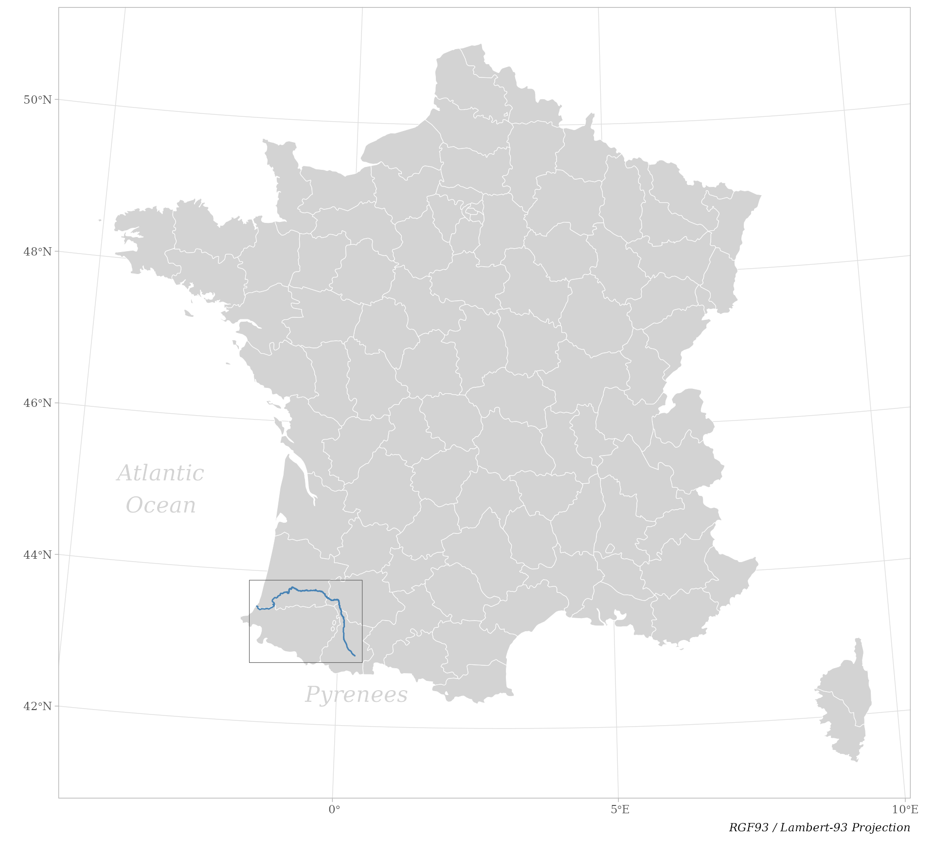
Figure 3. Location of the French river L’Adour
Along this river, a survey has been realized at three locations (Fig. 4). At each location, a sampling has been conducted on a regular grid composed of three transects each of them composed of five quadrats.
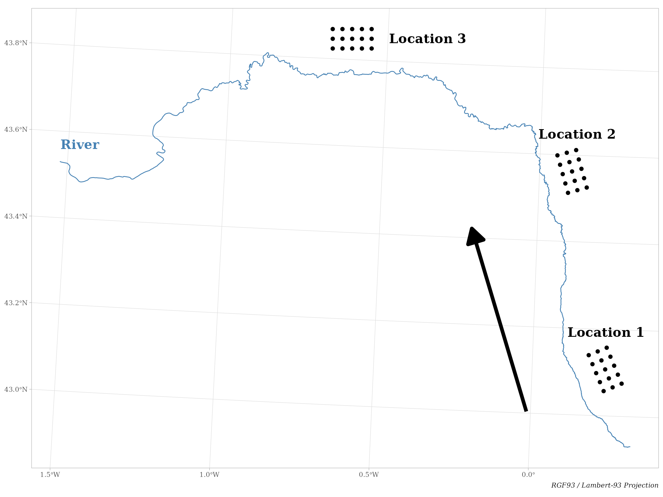
Figure 4. Survey sampling along the river L’Adour
The arrow in Fig. 4 indicates the direction of the river flow. This means that our sampling design is a directed spatial network (both inside a location and between locations) where the main direction is from upstream to downstream.
Let’s import this dataset provided by chessboard.
# Import data ----
path_to_file <- system.file("extdata", "adour_survey_sampling.csv",
                            package = "chessboard")

sampling  <- read.csv(path_to_file)

dim(sampling)
#> [1] 45  5
# First rows ----
head(sampling, 10)
#>    location transect quadrat longitude latitude
#> 1         1        1       1  474036.9  6221518
#> 2         1        1       2  473080.0  6223828
#> 3         1        1       3  472123.1  6226138
#> 4         1        1       4  471166.2  6228448
#> 5         1        1       5  470209.3  6230758
#> 6         1        2       1  476347.0  6222475
#> 7         1        2       2  475390.1  6224785
#> 8         1        2       3  474433.2  6227095
#> 9         1        2       4  473476.3  6229405
#> 10        1        2       5  472519.5  6231715
# Last rows ----
tail(sampling, 10)
#>    location transect quadrat longitude latitude
#> 36        3        2      11  414434.2  6312095
#> 37        3        2      12  411933.7  6312095
#> 38        3        2      13  409433.2  6312095
#> 39        3        2      14  406932.8  6312095
#> 40        3        2      15  404432.3  6312095
#> 41        3        3      11  414434.2  6314595
#> 42        3        3      12  411933.7  6314595
#> 43        3        3      13  409433.2  6314595
#> 44        3        3      14  406932.8  6314595
#> 45        3        3      15  404432.3  6314595
This data.frame contains the following columns:
-
location: the identifier of the location (numeric) -
transect: the identifier of the transect (numeric) -
quadrat: the identifier of the quadrat (numeric) -
longitude: the longitude of the site (node) defined in the RGF93 / Lambert-93 projection -
latitude: the latitude of the site (node) defined in the RGF93 / Lambert-93 projection
N.B. The column location is optional if
the survey has been conducted at one single location. If the network has
one dimension, one of the columns transect and
quadrat can be omitted. If the survey is not spatial, the
columns longitude and latitude can be
omitted.
Node labels
When working with chessboard, the first
step is to create node labels with the function
create_node_labels().
But first, let’s reduce the size of data by selecting the first location.
# Select the first location ----
sampling <- sampling[sampling$"location" == 1, ]

dim(sampling)
#> [1] 15  5
Let’s create node labels with the function
create_node_labels().
# Create node labels ----
nodes <- create_node_labels(data     = sampling,
                            location = "location",
                            transect = "transect",
                            quadrat  = "quadrat")

nodes
#>    node location transect quadrat longitude latitude
#> 1   1-1        1        1       1  474036.9  6221518
#> 2   1-2        1        1       2  473080.0  6223828
#> 3   1-3        1        1       3  472123.1  6226138
#> 4   1-4        1        1       4  471166.2  6228448
#> 5   1-5        1        1       5  470209.3  6230758
#> 6   2-1        1        2       1  476347.0  6222475
#> 7   2-2        1        2       2  475390.1  6224785
#> 8   2-3        1        2       3  474433.2  6227095
#> 9   2-4        1        2       4  473476.3  6229405
#> 10  2-5        1        2       5  472519.5  6231715
#> 11  3-1        1        3       1  478657.1  6223432
#> 12  3-2        1        3       2  477700.2  6225742
#> 13  3-3        1        3       3  476743.4  6228052
#> 14  3-4        1        3       4  475786.5  6230362
#> 15  3-5        1        3       5  474829.6  6232672
Node labels are a combination of the transect and the quadrat identifiers. They must be unique.
We can visualize this sampling on a Cartesian referential, i.e. non-spatial, where the x-axis corresponds to transects and the y-axis represents the quadrats (Fig. 5). This new referential is called a chessboard.
# Visualize chessboard ----
gg_chessboard(nodes)
Figure 5. Sampling survey as a chessboard
The function get_node_list() can be used to extract and
order the node list.
# Extract node labels ----
get_node_list(nodes)
#>  [1] "1-1" "1-2" "1-3" "1-4" "1-5" "2-1" "2-2" "2-3" "2-4" "2-5" "3-1" "3-2"
#> [13] "3-3" "3-4" "3-5"
Edge list
The creation of a list of edges (links) between nodes (sampling units) is based on the detection of neighbors.
In chessboard different methods have been implemented to
define neighborhood (argument method of the function
create_edge_list()). These methods are named
'pawn', 'rook', 'bishop',
'queen', etc. A complete list of available methods is
available at: https://frbcesab.github.io/chessboard/reference/index.html#detect-neighbors
Before using the function create_edge_list(), users can
explore these different methods by calling the functions
pawn(), rook(), bishop(),
queen(), etc. These functions only work on a specific node
(argument focus).
Let’s take a look of the neighborhood method pawn().
# Explore pawn method to find neighbors ----
neighbors_pawn <- pawn(nodes    = nodes,
                       focus    = "2-3",
                       degree   = 1,
                       directed = FALSE,
                       reverse  = FALSE)
neighbors_pawn
#>   node location transect quadrat longitude latitude
#> 1  2-2        1        2       2  475390.1  6224785
#> 2  2-4        1        2       4  473476.3  6229405
The package chessboard contains functions to visualize
detected neighbors on a chessboard: gg_chessboard() is used
to plot a chessboard (dimensions defined by the node list),
geom_node() emphasizes the focus node (in red), and
geom_neighbors() adds the detected neighbors (dots in
black).
gg_chessboard(nodes) +
  geom_node(nodes, focus = "2-3") +
  geom_neighbors(nodes, neighbors_pawn)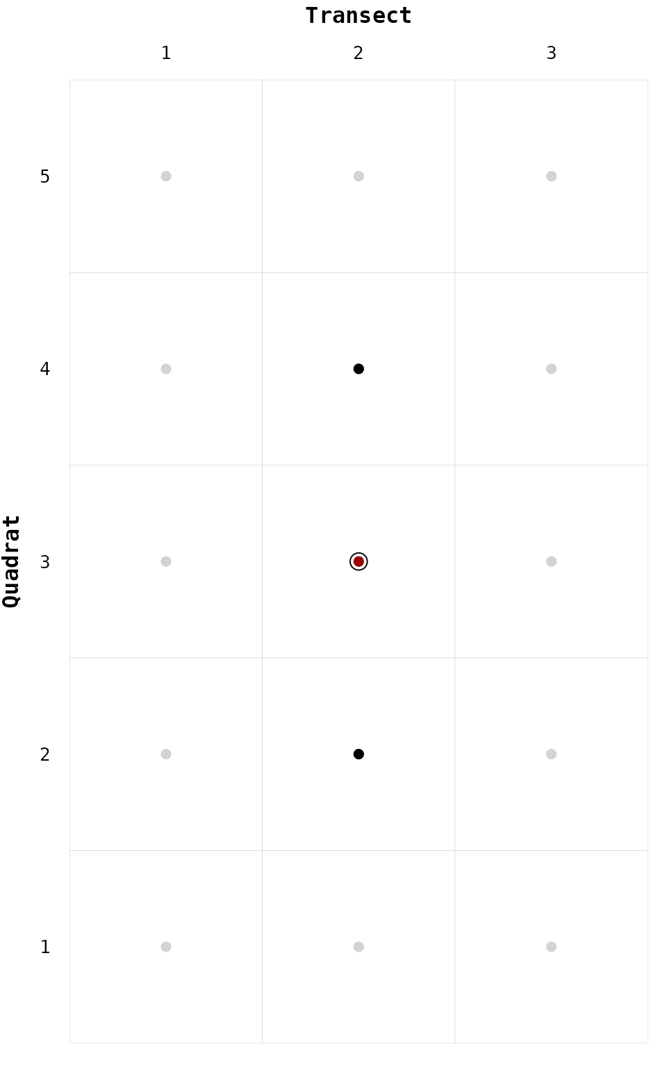
Figure 6. Detected neighbors (pawn method)
The function pawn() can detect neighbors vertically,
i.e. among quadrats along a transect. User can change the default
settings by increasing the degree of neighborhood
(degree = 4, Fig. 7A), by adding directionality
(directed = TRUE, Fig. 7B), and by reversing the default
directionality (directed = TRUE and
reverse = TRUE, Fig. 7C).
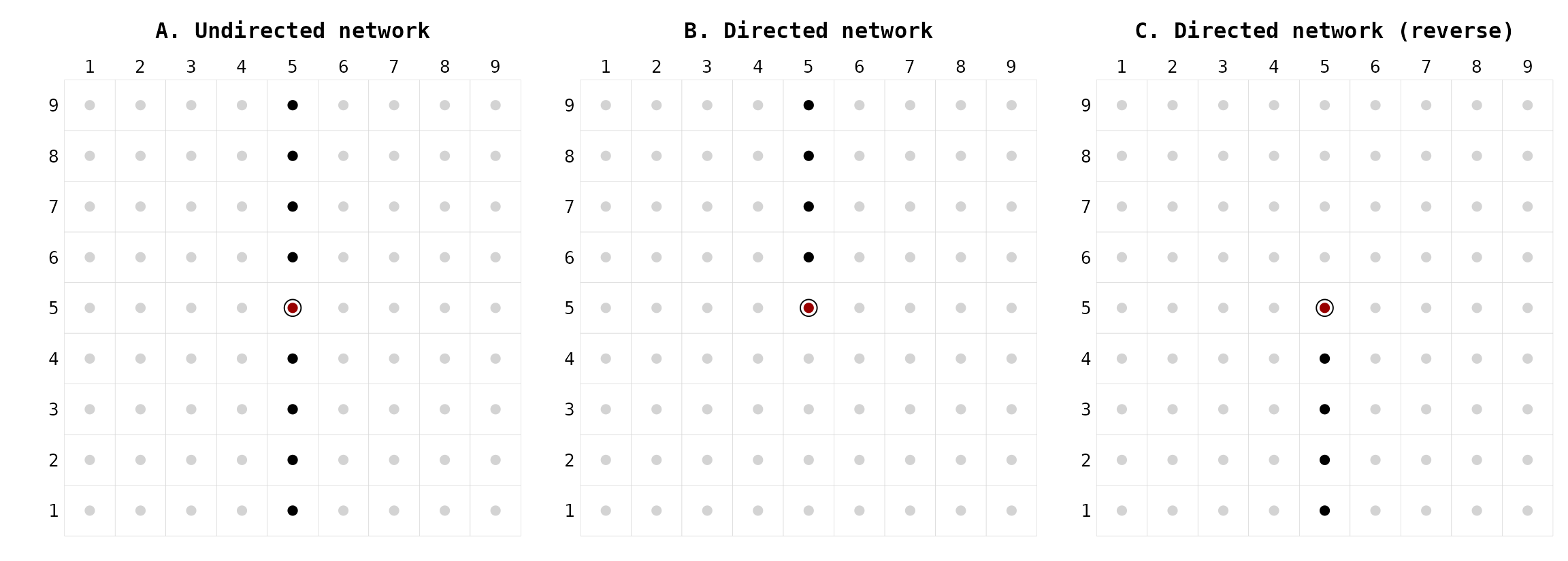
Figure 7. Pawn movements
Let’s take another example. The function bishop() can
detect neighbors diagonally. User can change the default settings by
increasing the degree of neighborhood (degree = 4, Fig.
8A), by adding directionality (directed = TRUE, Fig. 8B),
and by reversing the default directionality
(directed = TRUE and reverse = TRUE, Fig.
8C).
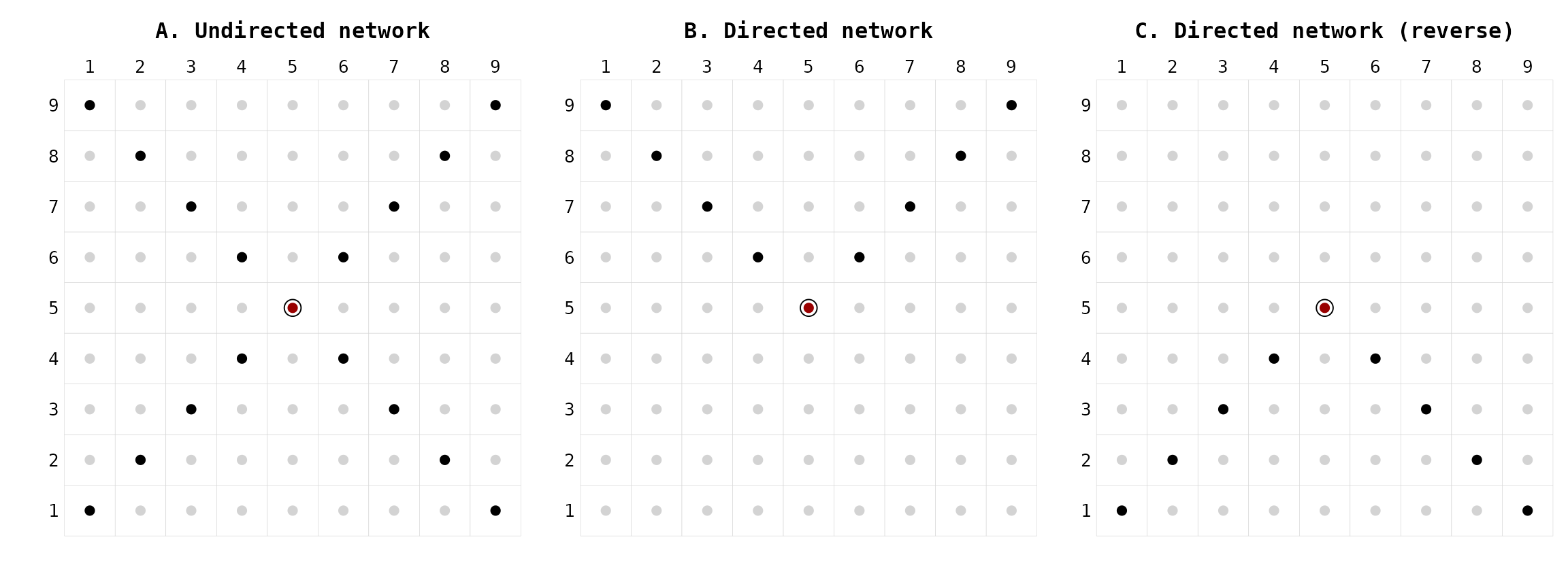
Figure 8. Bishop movements
The vignette Chess
pieces shows all possible methods available in
chessboard.
Now, let’s use the function create_edge_list() to create
an edge list using the method 'pawn' with a degree
1 of neighborhood and in a directional way.
# Create edge list ----
edges_pawn <- create_edge_list(nodes    = nodes,
                               method   = "pawn",
                               degree   = 1,
                               directed = TRUE,
                               reverse  = FALSE,
                               self     = FALSE)

edges_pawn
#>    from  to
#> 1   1-1 1-2
#> 2   1-2 1-3
#> 3   1-3 1-4
#> 4   1-4 1-5
#> 5   2-1 2-2
#> 6   2-2 2-3
#> 7   2-3 2-4
#> 8   2-4 2-5
#> 9   3-1 3-2
#> 10  3-2 3-3
#> 11  3-3 3-4
#> 12  3-4 3-5
It’s possible to visualize these edges on a map, i.e. by using
spatial coordinates. First, we need to convert our sites into a spatial
object (POINT).
# Convert nodes to sf object ----
nodes_sf <- sf::st_as_sf(nodes, coords = c("longitude", "latitude"),
                               crs = "epsg:2154")

head(nodes_sf)
#> Simple feature collection with 6 features and 4 fields
#> Geometry type: POINT
#> Dimension:     XY
#> Bounding box:  xmin: 470209.3 ymin: 6221518 xmax: 476347 ymax: 6230758
#> Projected CRS: RGF93 v1 / Lambert-93
#>   node location transect quadrat                 geometry
#> 1  1-1        1        1       1 POINT (474036.9 6221518)
#> 2  1-2        1        1       2   POINT (473080 6223828)
#> 3  1-3        1        1       3 POINT (472123.1 6226138)
#> 4  1-4        1        1       4 POINT (471166.2 6228448)
#> 5  1-5        1        1       5 POINT (470209.3 6230758)
#> 6  2-1        1        2       1   POINT (476347 6222475)
Now we can use the function edges_to_sf() to convert our
edge list into a spatial object (LINESTRING).
# Convert edge list to sf ----
edges_pawn_sf <- edges_to_sf(edges = edges_pawn,
                             sites = nodes_sf)

edges_pawn_sf
#> Simple feature collection with 12 features and 2 fields
#> Geometry type: LINESTRING
#> Dimension:     XY
#> Bounding box:  xmin: 470209.3 ymin: 6221518 xmax: 478657.1 ymax: 6232672
#> Projected CRS: RGF93 v1 / Lambert-93
#> First 10 features:
#>    from  to                       geometry
#> 1   1-1 1-2 LINESTRING (474036.9 622151...
#> 2   1-2 1-3 LINESTRING (473080 6223828,...
#> 3   1-3 1-4 LINESTRING (472123.1 622613...
#> 4   1-4 1-5 LINESTRING (471166.2 622844...
#> 5   2-1 2-2 LINESTRING (476347 6222475,...
#> 6   2-2 2-3 LINESTRING (475390.1 622478...
#> 7   2-3 2-4 LINESTRING (474433.2 622709...
#> 8   2-4 2-5 LINESTRING (473476.3 622940...
#> 9   3-1 3-2 LINESTRING (478657.1 622343...
#> 10  3-2 3-3 LINESTRING (477700.2 622574...
We can now map our nodes and edges.
# Map of nodes and edges ----
ggplot(nodes_sf) +
  geom_sf(size = 12) +
  geom_sf(data = edges_pawn_sf) +
  theme_light()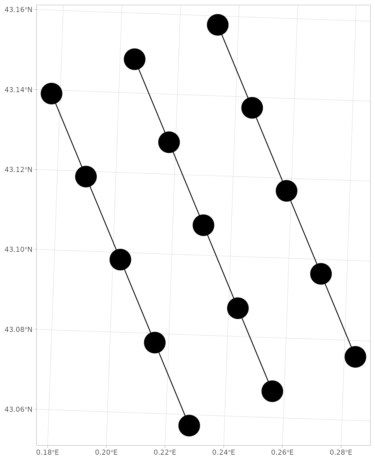
Figure 9. Edge list (pawn method)
Users may want to combine different methods to detect neighbors to
build complex scenarios. It’s possible by using for each method the
function create_edge_list() and using the function
append_edge_lists() to merge all edges in a single
list.
# Create edge list (Bishop method) ----
edges_bishop <- create_edge_list(nodes    = nodes,
                                 method   = "bishop",
                                 degree   = 1,
                                 directed = TRUE,
                                 reverse  = FALSE,
                                 self     = FALSE)

edges_bishop
#>    from  to
#> 1   1-1 2-2
#> 2   1-2 2-3
#> 3   1-3 2-4
#> 4   1-4 2-5
#> 5   2-1 1-2
#> 6   2-1 3-2
#> 7   2-2 1-3
#> 8   2-2 3-3
#> 9   2-3 1-4
#> 10  2-3 3-4
#> 11  2-4 1-5
#> 12  2-4 3-5
#> 13  3-1 2-2
#> 14  3-2 2-3
#> 15  3-3 2-4
#> 16  3-4 2-5

# Merge Pawn and Bishop edges ----
edges <- append_edge_lists(edges_pawn, edges_bishop)

# Convert edges to spatial layer ----
edges_sf <- edges_to_sf(edges, nodes_sf)
# Map of nodes and edges ----
ggplot(nodes_sf) +
  geom_sf(size = 12) +
  geom_sf(data = edges_sf) +
  theme_light()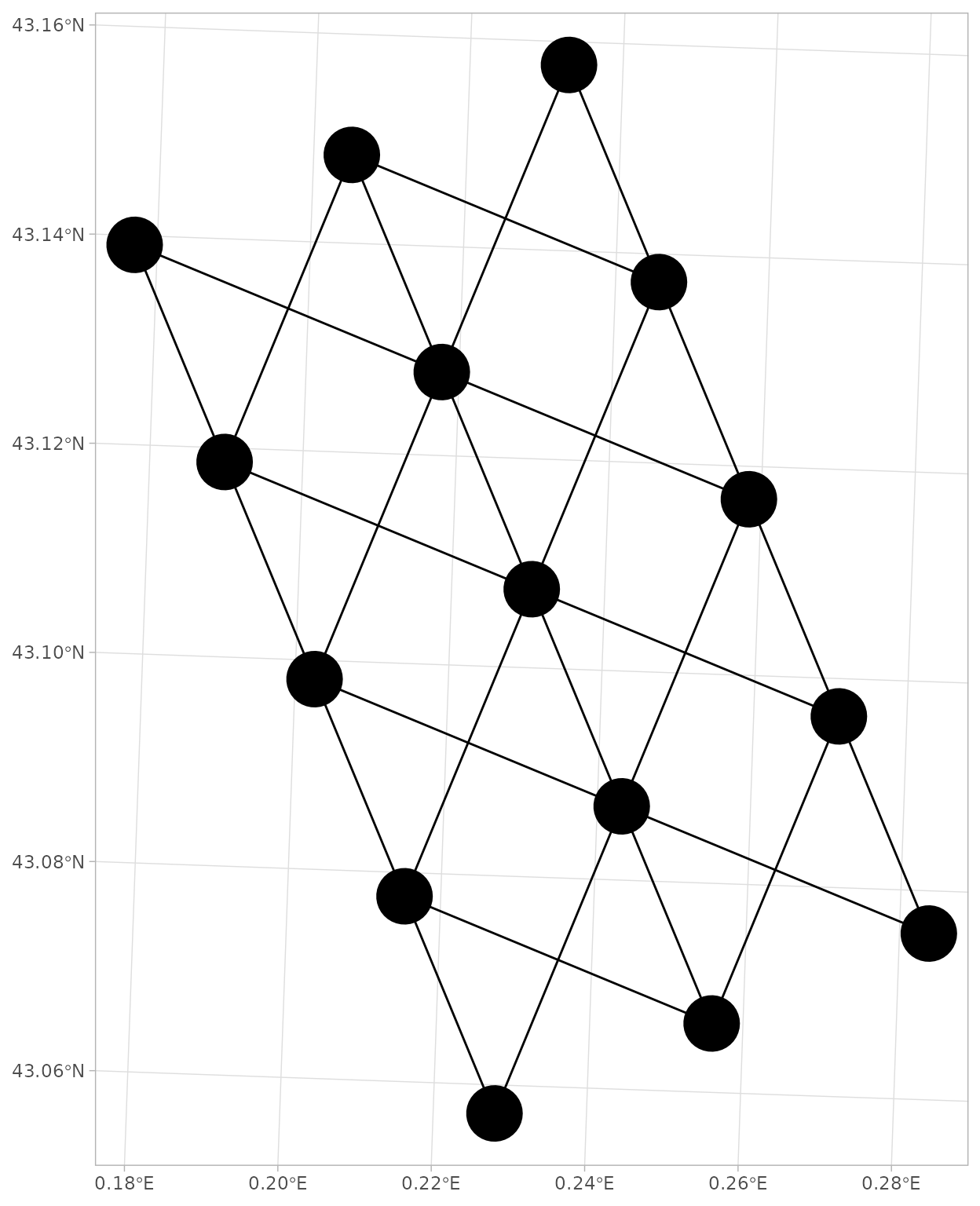
Figure 10. Edges list (combined methods)
Connectivity matrix
From this edge list, we can build a connectivity
matrix, i.e. a binary matrix of dimensions n x n,
where n is the number of nodes (sampling units) indicating
the presence (1) or the absence (0) of an edge
(link) between pairs of nodes.
We can use the function connectivity_matrix() of the
package chessboard.
# Create connectivity matrix ----
conn_matrix <- connectivity_matrix(edges)

conn_matrix
#>     1-1 1-2 1-3 1-4 1-5 2-1 2-2 2-3 2-4 2-5 3-1 3-2 3-3 3-4 3-5
#> 1-1   0   1   0   0   0   0   1   0   0   0   0   0   0   0   0
#> 1-2   0   0   1   0   0   0   0   1   0   0   0   0   0   0   0
#> 1-3   0   0   0   1   0   0   0   0   1   0   0   0   0   0   0
#> 1-4   0   0   0   0   1   0   0   0   0   1   0   0   0   0   0
#> 1-5   0   0   0   0   0   0   0   0   0   0   0   0   0   0   0
#> 2-1   0   1   0   0   0   0   1   0   0   0   0   1   0   0   0
#> 2-2   0   0   1   0   0   0   0   1   0   0   0   0   1   0   0
#> 2-3   0   0   0   1   0   0   0   0   1   0   0   0   0   1   0
#> 2-4   0   0   0   0   1   0   0   0   0   1   0   0   0   0   1
#> 2-5   0   0   0   0   0   0   0   0   0   0   0   0   0   0   0
#> 3-1   0   0   0   0   0   0   1   0   0   0   0   1   0   0   0
#> 3-2   0   0   0   0   0   0   0   1   0   0   0   0   1   0   0
#> 3-3   0   0   0   0   0   0   0   0   1   0   0   0   0   1   0
#> 3-4   0   0   0   0   0   0   0   0   0   1   0   0   0   0   1
#> 3-5   0   0   0   0   0   0   0   0   0   0   0   0   0   0   0
The package chessboard provides a function to visualize
this matrix: gg_matrix().
# Visualize connectivity matrix ----
gg_matrix(conn_matrix)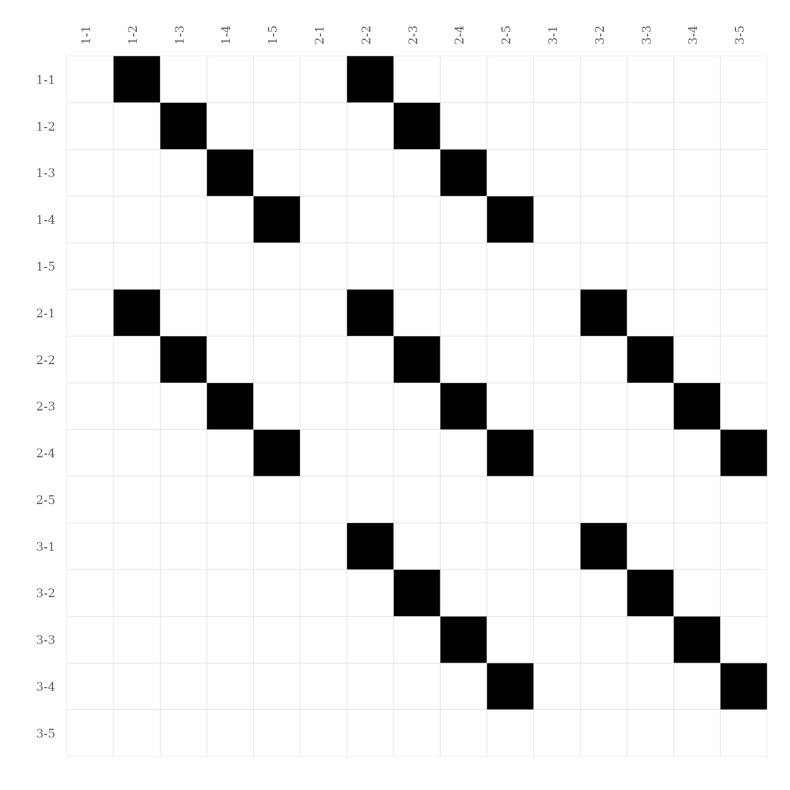
Figure 11. Connectivity matrix
Optionally, we can use the function
matrix_to_edge_list() to convert back the connectivity
matrix to edge list.
# Convert connectivity matrix to edge list ----
matrix_to_edge_list(conn_matrix)
#>    from  to edge
#> 1   1-1 1-2    1
#> 2   1-1 2-2    1
#> 3   1-2 1-3    1
#> 4   1-2 2-3    1
#> 5   1-3 1-4    1
#> 6   1-3 2-4    1
#> 7   1-4 1-5    1
#> 8   1-4 2-5    1
#> 9   2-1 1-2    1
#> 10  2-1 2-2    1
#> 11  2-1 3-2    1
#> 12  2-2 1-3    1
#> 13  2-2 2-3    1
#> 14  2-2 3-3    1
#> 15  2-3 1-4    1
#> 16  2-3 2-4    1
#> 17  2-3 3-4    1
#> 18  2-4 1-5    1
#> 19  2-4 2-5    1
#> 20  2-4 3-5    1
#> 21  3-1 2-2    1
#> 22  3-1 3-2    1
#> 23  3-2 2-3    1
#> 24  3-2 3-3    1
#> 25  3-3 2-4    1
#> 26  3-3 3-4    1
#> 27  3-4 2-5    1
#> 28  3-4 3-5    1
Extending chessboard
chessboard has been built to be compatible with the
following R packages: igraph (Csardi &
Nepusz 2006), sf (Pebesma
2018), and ggplot2 (Wickham
2016).
with sf
As seen before, the edge list can be converted into an spatial object
with the function edges_to_sf(). The output is an
sf LINESTRING that can be handled by many
functions of the package sf. For instance, let’s project
the coordinate system.
# Convert edges to spatial layer ----
edges_sf <- edges_to_sf(edges, nodes_sf)

# Project the CRS ----
edges_sf_lonlat <- sf::st_transform(edges_sf, crs = "epsg:4326")

# Check ----
edges_sf
#> Simple feature collection with 28 features and 2 fields
#> Geometry type: LINESTRING
#> Dimension:     XY
#> Bounding box:  xmin: 470209.3 ymin: 6221518 xmax: 478657.1 ymax: 6232672
#> Projected CRS: RGF93 v1 / Lambert-93
#> First 10 features:
#>    from  to                       geometry
#> 1   1-1 1-2 LINESTRING (474036.9 622151...
#> 2   1-1 2-2 LINESTRING (474036.9 622151...
#> 3   1-2 1-3 LINESTRING (473080 6223828,...
#> 4   1-2 2-3 LINESTRING (473080 6223828,...
#> 5   1-3 1-4 LINESTRING (472123.1 622613...
#> 6   1-3 2-4 LINESTRING (472123.1 622613...
#> 7   1-4 1-5 LINESTRING (471166.2 622844...
#> 8   1-4 2-5 LINESTRING (471166.2 622844...
#> 9   2-1 1-2 LINESTRING (476347 6222475,...
#> 10  2-1 2-2 LINESTRING (476347 6222475,...
edges_sf_lonlat
#> Simple feature collection with 28 features and 2 fields
#> Geometry type: LINESTRING
#> Dimension:     XY
#> Bounding box:  xmin: 0.1770395 ymin: 43.05727 xmax: 0.2838317 ymax: 43.15778
#> Geodetic CRS:  WGS 84
#> First 10 features:
#>    from  to                       geometry
#> 1   1-1 1-2 LINESTRING (0.2280052 43.05...
#> 2   1-1 2-2 LINESTRING (0.2280052 43.05...
#> 3   1-2 1-3 LINESTRING (0.2152773 43.07...
#> 4   1-2 2-3 LINESTRING (0.2152773 43.07...
#> 5   1-3 1-4 LINESTRING (0.2025404 43.09...
#> 6   1-3 2-4 LINESTRING (0.2025404 43.09...
#> 7   1-4 1-5 LINESTRING (0.1897944 43.11...
#> 8   1-4 2-5 LINESTRING (0.1897944 43.11...
#> 9   2-1 1-2 LINESTRING (0.2559139 43.06...
#> 10  2-1 2-2 LINESTRING (0.2559139 43.06...
User can also export this spatial layer.
# Export layer as a GeoPackage ----
sf::st_write(edges_sf, "edge_list.gpkg")
For more information about the package sf, please visit
the manual.
with ggplot2
All plotting functions in chessboard are produced with
the ggplot2 engine and are highly customizable. For
instance, let’s change the default theme.
# Change default ggplot2 theme ----
gg_matrix(conn_matrix) +
  theme_bw() +
  theme(legend.position = "none")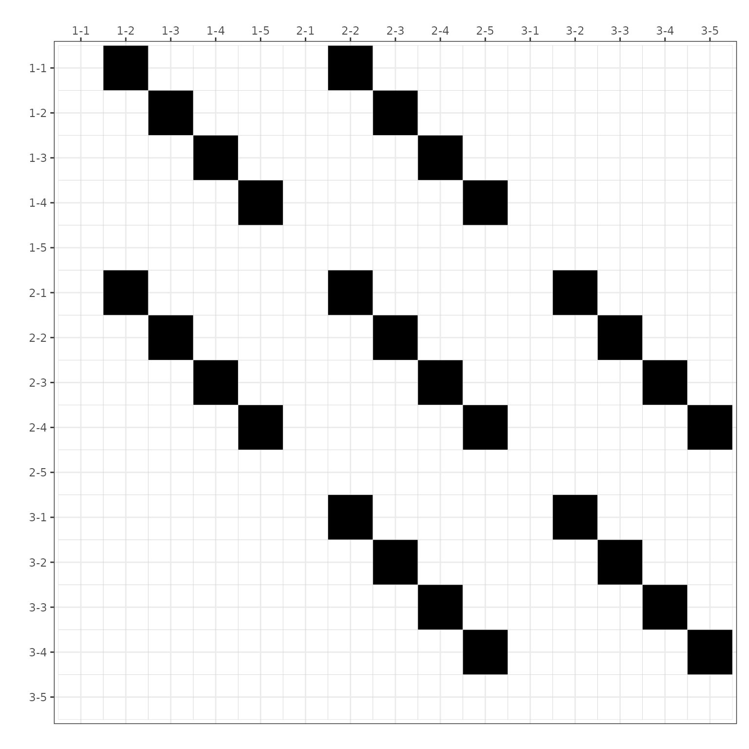
Figure 12. Custom connectivity matrix
For more information about the package ggplot2, please
visit the manual.
with igraph
The package igraph is commonly use to analyze network
data. User can use the function
igraph::graph_from_data_frame() to convert the edge list
created with chessboard to an igraph
object.
# Convert edge list to igraph object ----
igraph_obj <- igraph::graph_from_data_frame(d        = edges,
                                            directed = TRUE,
                                            vertices = nodes)

# Check -----
class(igraph_obj)
#> [1] "igraph"

print(igraph_obj)
#> IGRAPH 1c8828a DN-- 15 28 --
#> + attr: name (v/c), location (v/n), transect (v/n), quadrat (v/n),
#> | longitude (v/n), latitude (v/n)
#> + edges from 1c8828a (vertex names):
#>  [1] 1-1->1-2 1-1->2-2 1-2->1-3 1-2->2-3 1-3->1-4 1-3->2-4 1-4->1-5 1-4->2-5
#>  [9] 2-1->1-2 2-1->2-2 2-1->3-2 2-2->1-3 2-2->2-3 2-2->3-3 2-3->1-4 2-3->2-4
#> [17] 2-3->3-4 2-4->1-5 2-4->2-5 2-4->3-5 3-1->2-2 3-1->3-2 3-2->2-3 3-2->3-3
#> [25] 3-3->2-4 3-3->3-4 3-4->2-5 3-4->3-5
Let’s plot our network using igraph.
# Plot the network w/ igraph ----
plot(igraph_obj)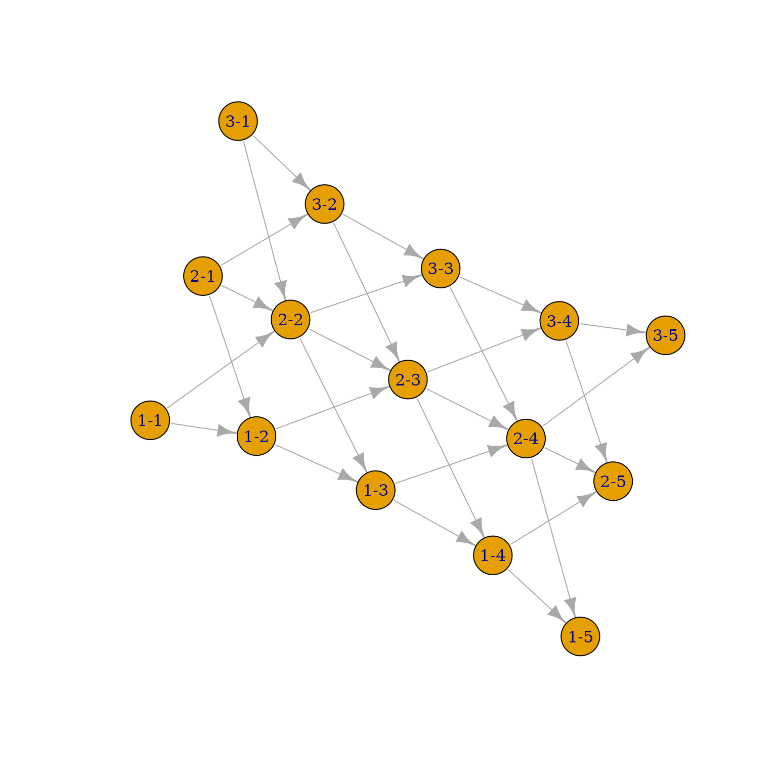
Figure 13. Network visualization w/ igraph
For more information about the package igraph, please
visit the manual.
References
Bivand R & Wong D (2018) Comparing implementations of global and local indicators of spatial association. TEST, 27, 716–748. https://doi.org/10.1007/s11749-018-0599-x.
Csardi G & Nepusz T (2006) The igraph software package for complex network research. InterJournal, Complex Systems, 1695, 1–9. https://igraph.org/.
Pebesma E (2018) Simple Features for R: Standardized support for spatial vector data. The R Journal, 10, 439–446. https://doi.org/10.32614/RJ-2018-009.
Wickham H (2016) ggplot2: Elegant graphics for data analysis (p. 213). Springer-Verlag. https://ggplot2.tidyverse.org/.