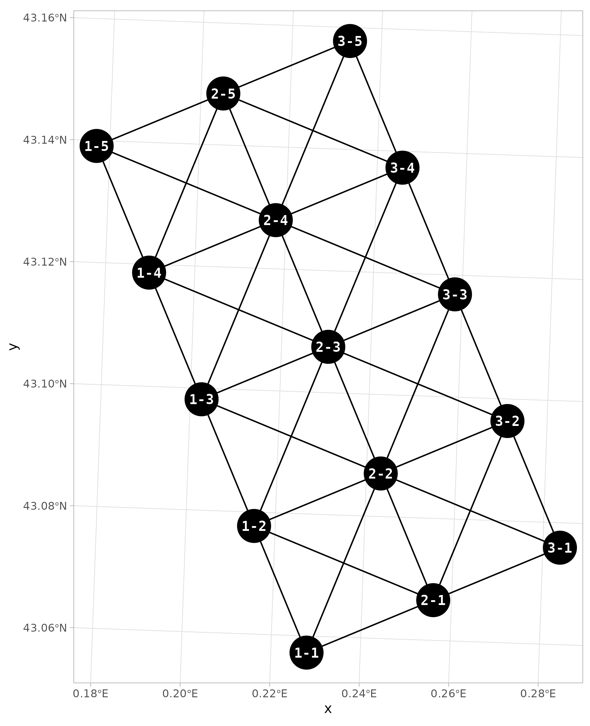
The package chessboard provides some plotting functions
to:
- visualize data on a chessboard
- visualize matrices
- visualize data on a map
All these functions have been implemented using the ggplot2 package,
meaning that they are highly customizable.
# Setup ----
library("chessboard")
library("ggplot2")
To illustrate these plotting functions, let’s import the data
provided by chessboard (see the Get
started vignette for a full description).
# Location of the data ----
path_to_file <- system.file("extdata", "adour_survey_sampling.csv",
                            package = "chessboard")

# Read the data ----
sampling  <- read.csv(path_to_file)

head(sampling)
#>   location transect quadrat longitude latitude
#> 1        1        1       1  474036.9  6221518
#> 2        1        1       2  473080.0  6223828
#> 3        1        1       3  472123.1  6226138
#> 4        1        1       4  471166.2  6228448
#> 5        1        1       5  470209.3  6230758
#> 6        1        2       1  476347.0  6222475
For the purpose of this vignette, let’s subset the first location.
# Subset location 1 ----
sampling <- sampling[sampling$"location" == 1, ]

sampling
#>    location transect quadrat longitude latitude
#> 1         1        1       1  474036.9  6221518
#> 2         1        1       2  473080.0  6223828
#> 3         1        1       3  472123.1  6226138
#> 4         1        1       4  471166.2  6228448
#> 5         1        1       5  470209.3  6230758
#> 6         1        2       1  476347.0  6222475
#> 7         1        2       2  475390.1  6224785
#> 8         1        2       3  474433.2  6227095
#> 9         1        2       4  473476.3  6229405
#> 10        1        2       5  472519.5  6231715
#> 11        1        3       1  478657.1  6223432
#> 12        1        3       2  477700.2  6225742
#> 13        1        3       3  476743.4  6228052
#> 14        1        3       4  475786.5  6230362
#> 15        1        3       5  474829.6  6232672
The sampling is a grid of dimensions 3 transects x 5 quadrats.
When working with chessboard, the first step is to
create node labels with the function
create_node_labels().
# Create node labels ----
nodes <- create_node_labels(data     = sampling,
                            location = "location",
                            transect = "transect",
                            quadrat  = "quadrat")

nodes
#>    node location transect quadrat longitude latitude
#> 1   1-1        1        1       1  474036.9  6221518
#> 2   1-2        1        1       2  473080.0  6223828
#> 3   1-3        1        1       3  472123.1  6226138
#> 4   1-4        1        1       4  471166.2  6228448
#> 5   1-5        1        1       5  470209.3  6230758
#> 6   2-1        1        2       1  476347.0  6222475
#> 7   2-2        1        2       2  475390.1  6224785
#> 8   2-3        1        2       3  474433.2  6227095
#> 9   2-4        1        2       4  473476.3  6229405
#> 10  2-5        1        2       5  472519.5  6231715
#> 11  3-1        1        3       1  478657.1  6223432
#> 12  3-2        1        3       2  477700.2  6225742
#> 13  3-3        1        3       3  476743.4  6228052
#> 14  3-4        1        3       4  475786.5  6230362
#> 15  3-5        1        3       5  474829.6  6232672
Visualizing chessboard
gg_chessboard
The first plotting function to use is gg_chessboard():
it will plot the (spatial) sampling as a chessboard, i.e. two-dimension
grid where the x-axis is the transect and the y-axis is the quadrat.
# Plot the sampling as a chessboard ----
gg_chessboard(nodes)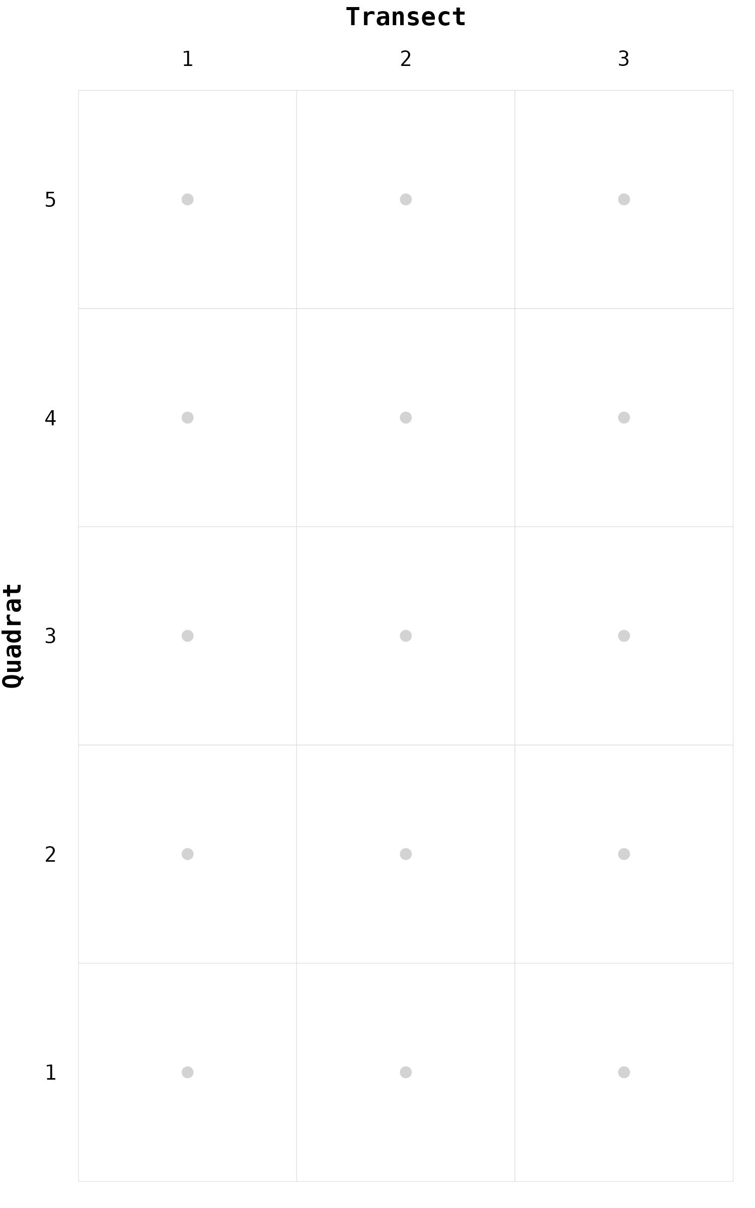
geom_node
On this chessboard, we can locate one specific node using the
function geom_node().
# Locate one node ----
gg_chessboard(nodes) +
  geom_node(nodes, focus = "2-3")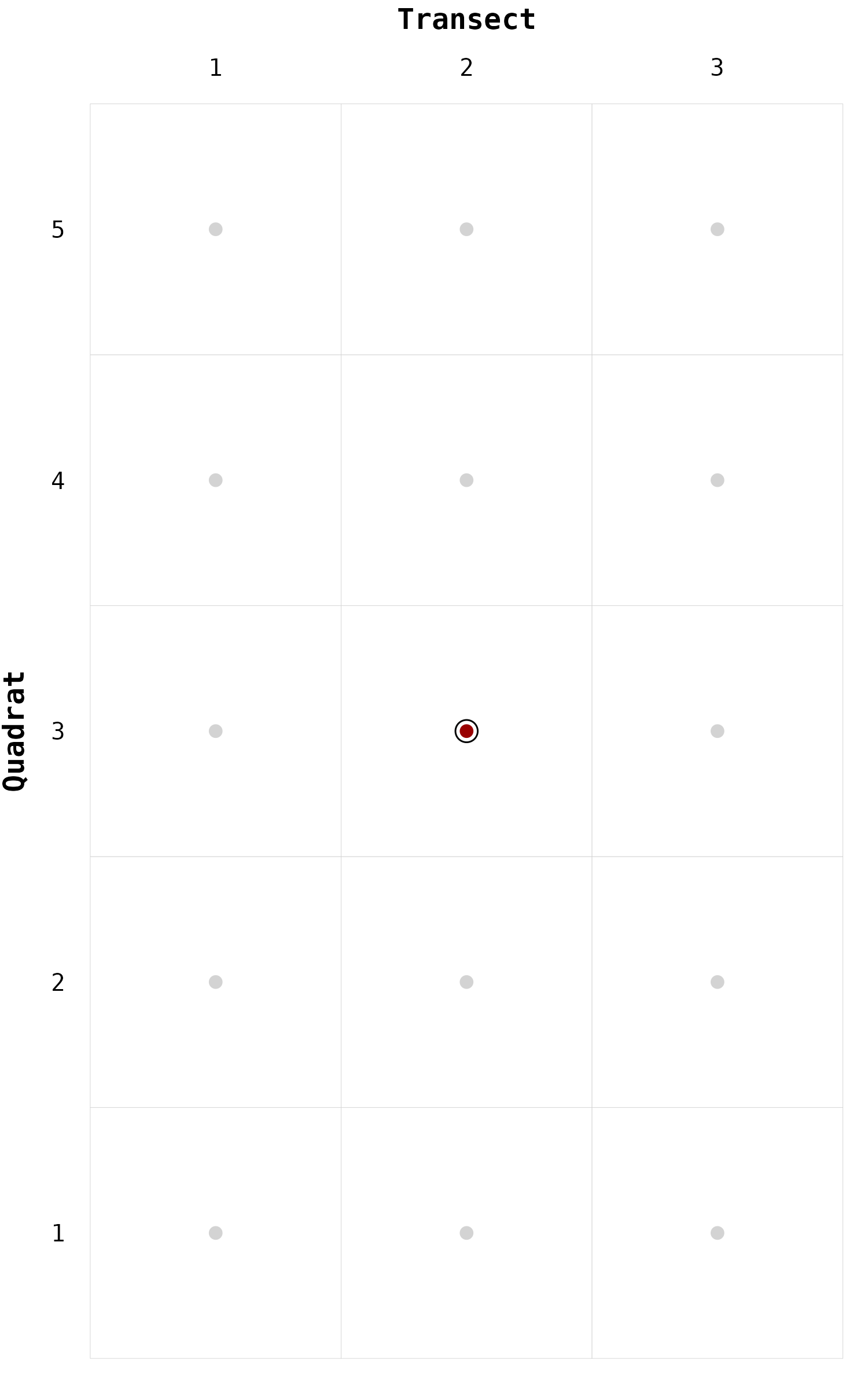
We can call the function geom_node() several times to
emphase various nodes.
# Locate various nodes ----
gg_chessboard(nodes) +
  geom_node(nodes, focus = "2-3") +
  geom_node(nodes, focus = "1-5") +
  geom_node(nodes, focus = "3-1")
geom_neighbors
As mentioned in the Get
started vignette, we can test the neighbors detection of a specific
node by using the functions pawn(), fool(),
rook(), etc.
Let’s apply the function rook() on the node
2-3.
# Neighbors detection ----
nb_rook <- rook(nodes, focus = "2-3")

nb_rook
#>   node location transect quadrat longitude latitude
#> 1  1-3        1        1       3  472123.1  6226138
#> 2  2-2        1        2       2  475390.1  6224785
#> 3  2-4        1        2       4  473476.3  6229405
#> 4  3-3        1        3       3  476743.4  6228052
Let’s visualize these neighbors on a chessboard by using the function
geom_neighbors().
# Locate neighbors ----
gg_chessboard(nodes) +
  geom_node(nodes, focus = "2-3") +
  geom_neighbors(nodes, neighbors = nb_rook)
geom_edges
Instead of plotting the neighbors, we can directly plot the edges
using the function geom_edges(). This function has the
advantage to show the direction of the edges.
# Locate neighbors ----
gg_chessboard(nodes) +
  geom_edges(nodes, focus = "2-3", neighbors = nb_rook) +
  geom_node(nodes, focus = "2-3")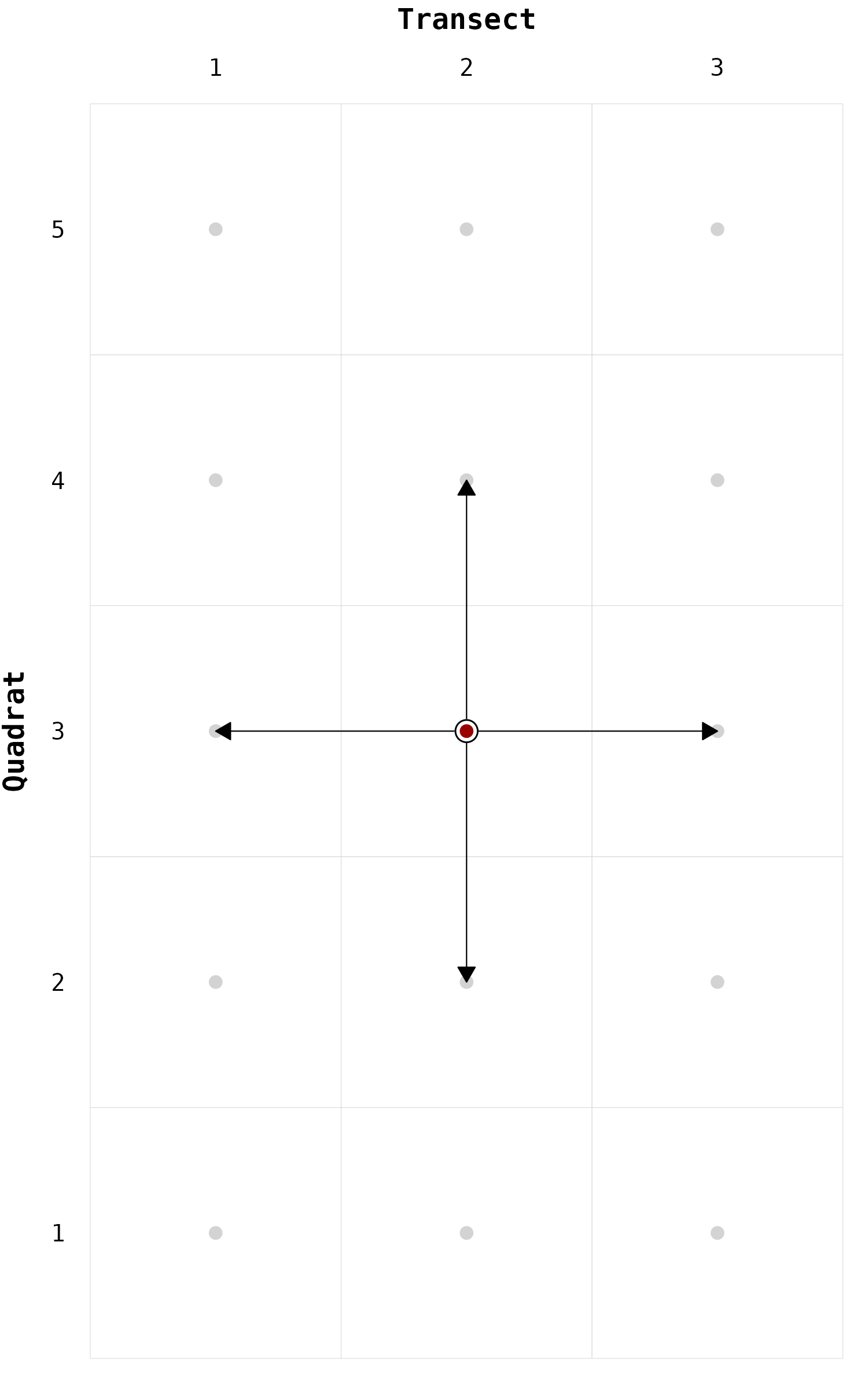
Now let’s call the function bishop() to create a second
edge list.
# Neighbors detection ----
nb_bishop <- bishop(nodes, focus = "2-3")

nb_bishop
#>   node location transect quadrat longitude latitude
#> 1  1-2        1        1       2  473080.0  6223828
#> 2  1-4        1        1       4  471166.2  6228448
#> 3  3-2        1        3       2  477700.2  6225742
#> 4  3-4        1        3       4  475786.5  6230362
As for the function geom_node(), we can call the
functions geom_edges() and geom_neighbors()
several times.
# Locate neighbors ----
gg_chessboard(nodes) +
  geom_edges(nodes, focus = "2-3", neighbors = nb_rook) +
  geom_edges(nodes, focus = "2-3", neighbors = nb_bishop) +
  geom_neighbors(nodes, neighbors = nb_rook) +
  geom_neighbors(nodes, neighbors = nb_bishop) +
  geom_node(nodes, focus = "2-3")
Plotting matrices
These two previous moves (rook and bishop) combined together are equivalent to the queen. For the rest of the vignette let’s create the edge list using the queen move.
# Edges list ----
edges <- create_edge_list(nodes, method = "queen")

head(edges)
#>   from  to
#> 1  1-1 1-2
#> 2  1-1 2-1
#> 3  1-1 2-2
#> 4  1-2 1-1
#> 5  1-2 1-3
#> 6  1-2 2-1
From this edge list, we can build the associated connectivity matrix
with the function connectivity_matrix().
# Connectivity matrix ----
mat <- connectivity_matrix(edges)

mat
#>     1-1 1-2 1-3 1-4 1-5 2-1 2-2 2-3 2-4 2-5 3-1 3-2 3-3 3-4 3-5
#> 1-1   0   1   0   0   0   1   1   0   0   0   0   0   0   0   0
#> 1-2   1   0   1   0   0   1   1   1   0   0   0   0   0   0   0
#> 1-3   0   1   0   1   0   0   1   1   1   0   0   0   0   0   0
#> 1-4   0   0   1   0   1   0   0   1   1   1   0   0   0   0   0
#> 1-5   0   0   0   1   0   0   0   0   1   1   0   0   0   0   0
#> 2-1   1   1   0   0   0   0   1   0   0   0   1   1   0   0   0
#> 2-2   1   1   1   0   0   1   0   1   0   0   1   1   1   0   0
#> 2-3   0   1   1   1   0   0   1   0   1   0   0   1   1   1   0
#> 2-4   0   0   1   1   1   0   0   1   0   1   0   0   1   1   1
#> 2-5   0   0   0   1   1   0   0   0   1   0   0   0   0   1   1
#> 3-1   0   0   0   0   0   1   1   0   0   0   0   1   0   0   0
#> 3-2   0   0   0   0   0   1   1   1   0   0   1   0   1   0   0
#> 3-3   0   0   0   0   0   0   1   1   1   0   0   1   0   1   0
#> 3-4   0   0   0   0   0   0   0   1   1   1   0   0   1   0   1
#> 3-5   0   0   0   0   0   0   0   0   1   1   0   0   0   1   0
A better way to visualize any kind of matrices, is to call the
function gg_matrix().
# Visualize matrix ----
gg_matrix(mat)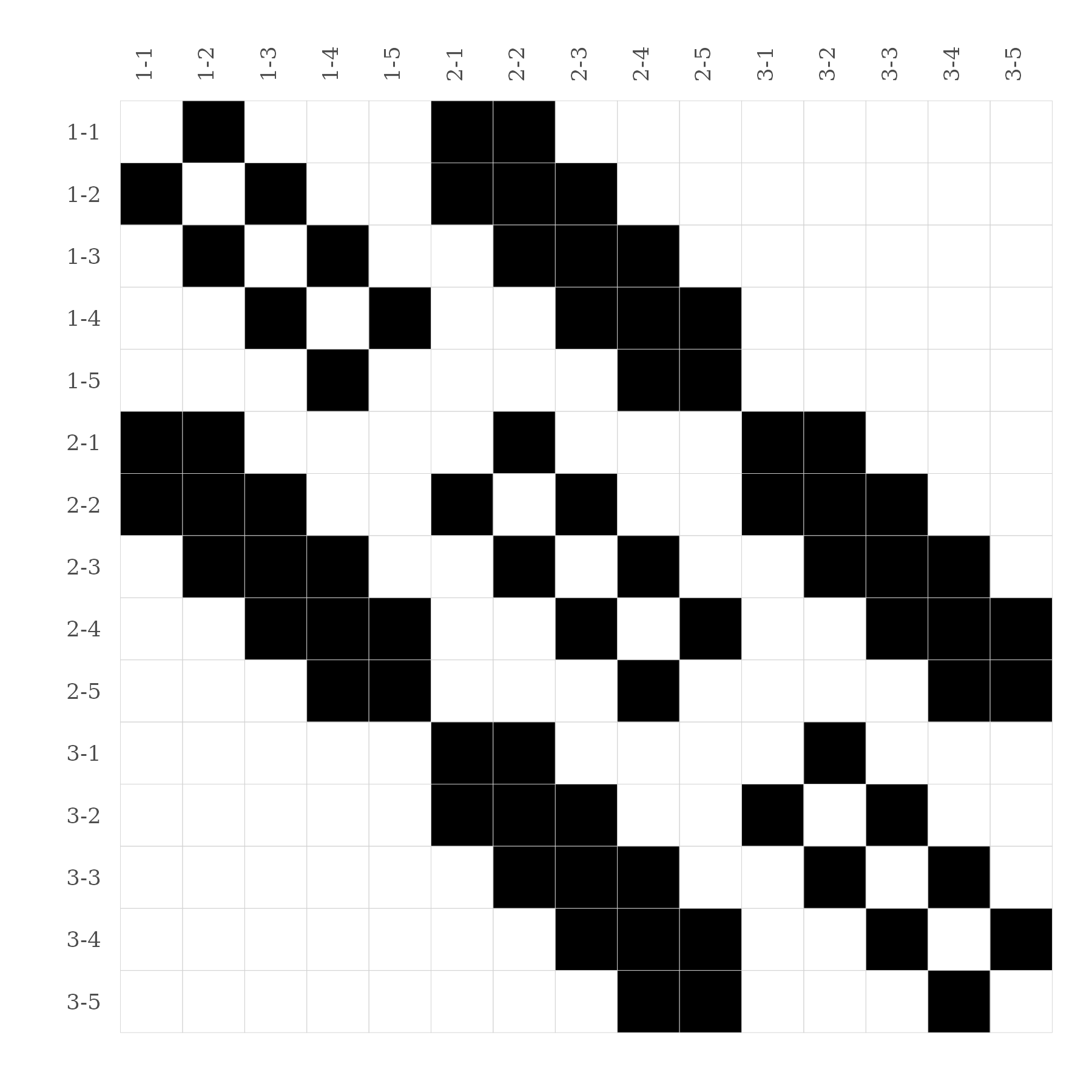
Mapping edges
Now, let’s go back into a spatial world. First let’s convert our
sampling into an sf object.
# Convert sampling to sf object ----
nodes_sf <- sf::st_as_sf(nodes,
                         coords = c("longitude", "latitude"),
                         crs = "epsg:2154")

nodes_sf
#> Simple feature collection with 15 features and 4 fields
#> Geometry type: POINT
#> Dimension:     XY
#> Bounding box:  xmin: 470209.3 ymin: 6221518 xmax: 478657.1 ymax: 6232672
#> Projected CRS: RGF93 v1 / Lambert-93
#> First 10 features:
#>    node location transect quadrat                 geometry
#> 1   1-1        1        1       1 POINT (474036.9 6221518)
#> 2   1-2        1        1       2   POINT (473080 6223828)
#> 3   1-3        1        1       3 POINT (472123.1 6226138)
#> 4   1-4        1        1       4 POINT (471166.2 6228448)
#> 5   1-5        1        1       5 POINT (470209.3 6230758)
#> 6   2-1        1        2       1   POINT (476347 6222475)
#> 7   2-2        1        2       2 POINT (475390.1 6224785)
#> 8   2-3        1        2       3 POINT (474433.2 6227095)
#> 9   2-4        1        2       4 POINT (473476.3 6229405)
#> 10  2-5        1        2       5 POINT (472519.5 6231715)
To convert our edge list into a spatial object, we can use the
function edges_to_sf().
# Convert edges to sf object ----
edges_sf <- edges_to_sf(edges, nodes_sf)

edges_sf
#> Simple feature collection with 76 features and 2 fields
#> Geometry type: LINESTRING
#> Dimension:     XY
#> Bounding box:  xmin: 470209.3 ymin: 6221518 xmax: 478657.1 ymax: 6232672
#> Projected CRS: RGF93 v1 / Lambert-93
#> First 10 features:
#>    from  to                       geometry
#> 1   1-1 1-2 LINESTRING (474036.9 622151...
#> 2   1-1 2-1 LINESTRING (474036.9 622151...
#> 3   1-1 2-2 LINESTRING (474036.9 622151...
#> 4   1-2 1-1 LINESTRING (473080 6223828,...
#> 5   1-2 1-3 LINESTRING (473080 6223828,...
#> 6   1-2 2-1 LINESTRING (473080 6223828,...
#> 7   1-2 2-2 LINESTRING (473080 6223828,...
#> 8   1-2 2-3 LINESTRING (473080 6223828,...
#> 9   1-3 1-2 LINESTRING (472123.1 622613...
#> 10  1-3 1-4 LINESTRING (472123.1 622613...
The result is a collection of LINESTRINGS, i.e. a
collection of spatial lines where each line is an edge defined in the
coordinate system (CRS) of the sampling.
Let’s use ggplot2 and sf to map the nodes
and the edges.
# Map of nodes and edges ----
ggplot() +
  geom_sf(data = edges_sf) +
  geom_sf(data = nodes_sf, size = 12) +
  theme_light()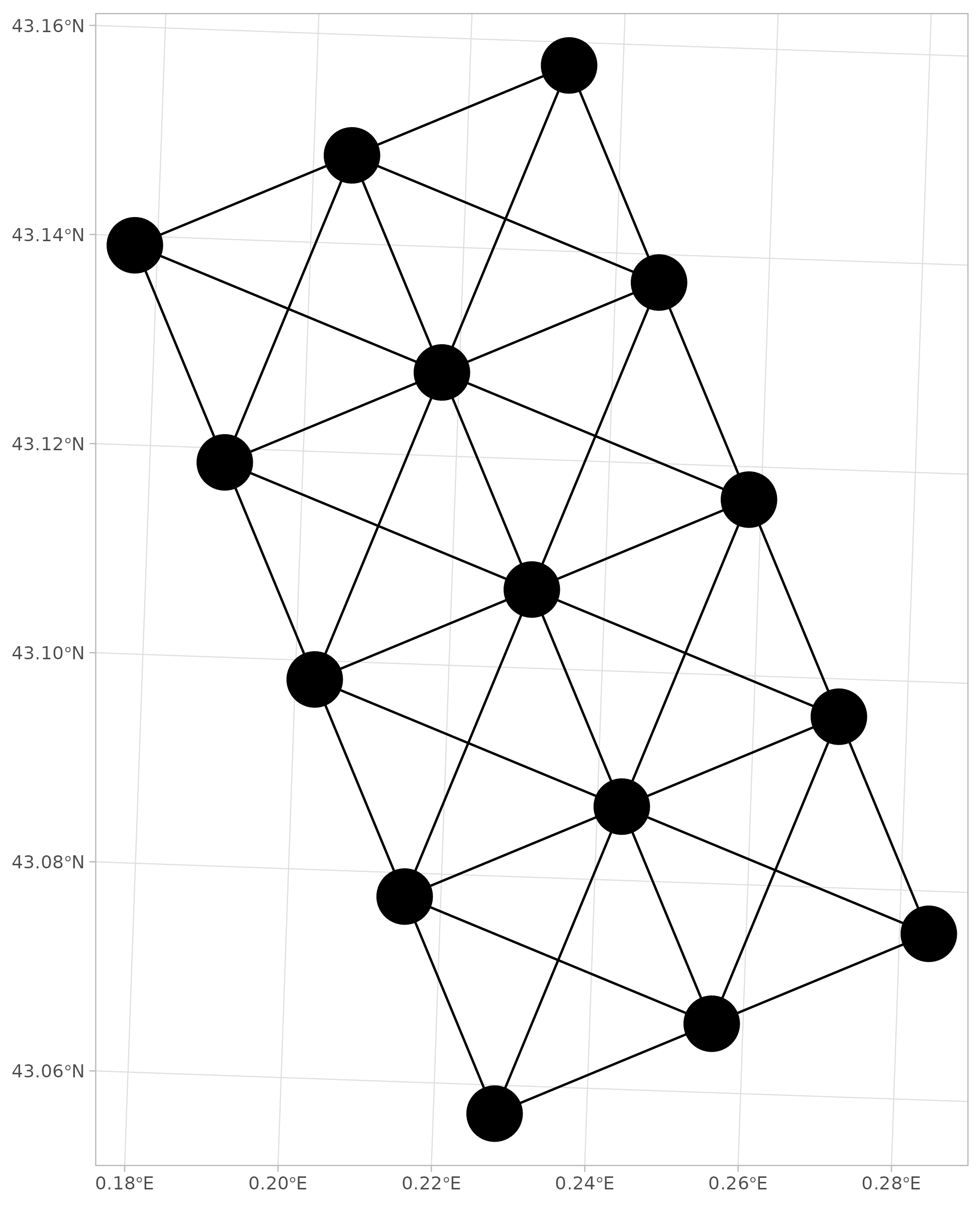
Finally, let’s add the node labels on this map.
# Map of nodes and edges ----
ggplot() +
  geom_sf(data = edges_sf) +
  geom_sf(data = nodes_sf, size = 12) +
  geom_sf_text(data = nodes_sf, aes(label = node),
               color = "white", fontface = "bold",
               family = "mono") +
  theme_light()